Log-Normal Distribution
March 29, 2018
Getting Started
Power Spectral Density
Converting Recorded Data
Statistics & Probabilities
Test Control
Back to: Random Testing
Many physical phenomena exhibit log-normal distribution. When a system’s response amplitude is the product of multiple independent parameters, the distribution of the response amplitude tends to be log-normal.
The log of the amplitude is the sum of the logs of the multiplicative terms. The central limit theorem implies that the log of the amplitude will have a normal distribution.
For example, if x = A·B/C, then log(x) = log(A) + log(B) – log(C), with A, B, C positive values. Figure 3.23 shows the log-normal distribution plotted on both a linear and log x scale.
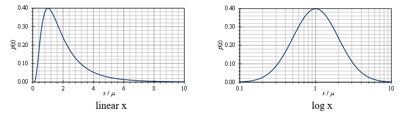
Figure 3.23. Log-Normal distribution on a linear and log x scale.
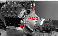
In random vibration, this applies to the distribution of the vibration magnitude over an ensemble of random conditions. Figure 3.24 displays a histogram of the RMS acceleration levels (ARMS) measured in the vertical and transverse directions on the coupling housing of 40 nominally identical diesel engines running under nominally identical conditions.
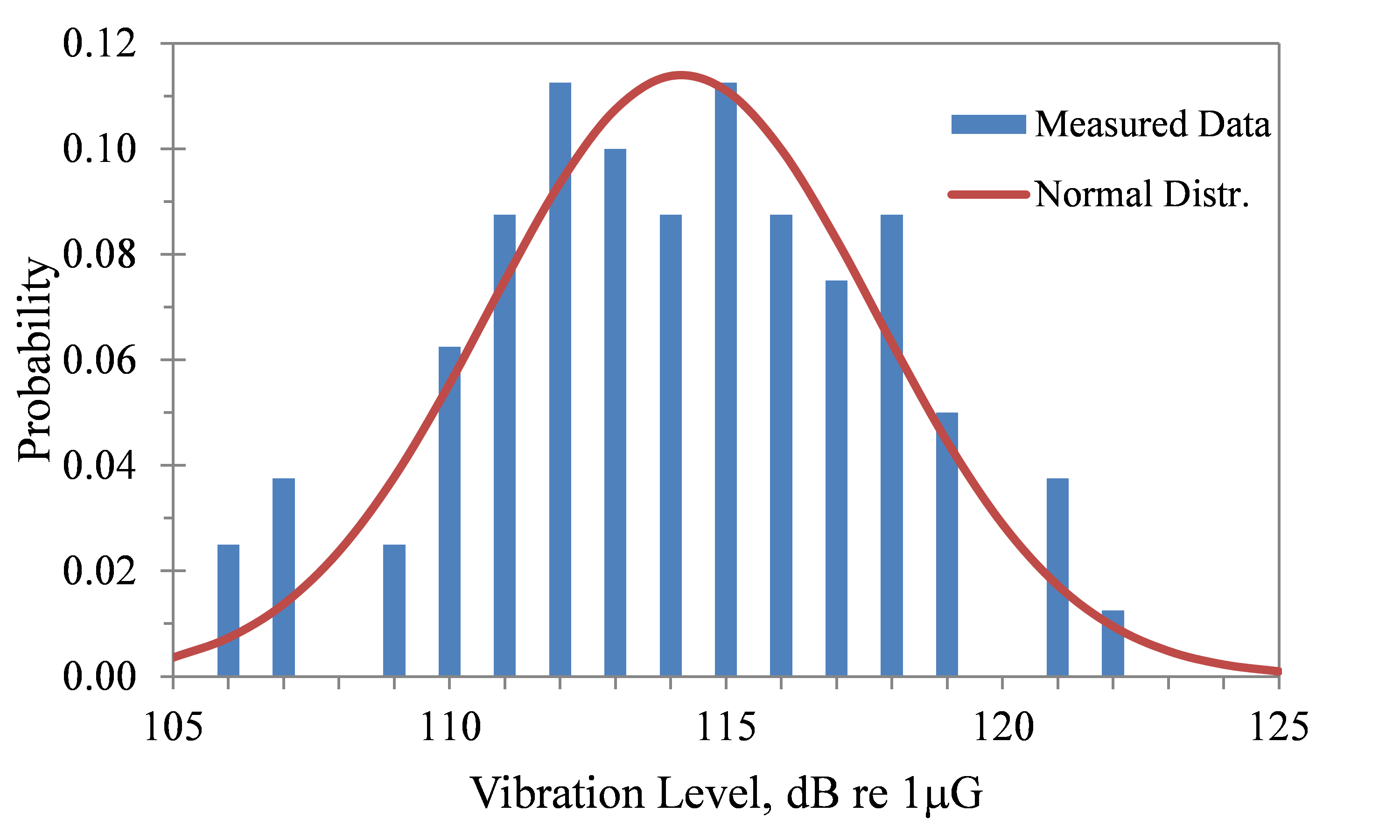
Figure 3.24. Distribution of engine vibration levels.
The measured data are plotted on a decibel scale [decibel level = 20 Log (ARMS/1 μG), dB], and compared to a normal distribution of the Log levels with a mean of 114.2 dB and σ = 3.5 dB.