Windowing
March 29, 2018
Getting Started
Power Spectral Density
Converting Recorded Data
Statistics & Probabilities
Test Control
Back to: Random Testing
The Fourier series assumes a signal is periodic in time T. When a signal is digitized into N samples from 0 to N – 1, the Fourier series concludes that the next sample (N) will be the same value as the first (0).
This scenario is not the case for most vibration signals. Therefore, a discontinuity usually exists between the end of the digitized signal and the beginning of the presumed periodic repetition. This discontinuity causes the fast Fourier transform (FFT) algorithm to generate artificial noise.
Discontinuity and Leakage
Figure 2.19 illustrates this discontinuity using a simple case of two sine waves. The first wave fits in the sampled time T = 0.512 sec. with an integer number of cycles (periodic in time). The second is slightly off (non-periodic in time), which generates a discontinuity in time and noise in the FFT.
The theoretical power spectral density (PSD) of a sine wave is an impulse at its frequency. The discontinuity resulting from the non-periodic signal generates spurious amplitudes in the adjacent frequencies called leakage.
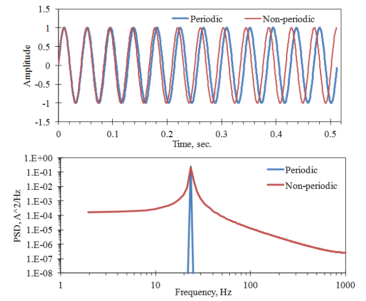
Figure 2.19. The effect of periodic and non-periodic signals (in Time T) on the FFT computation. SR = 2000 samples/sec., N = 1024, Periodic: 23.4375 Hz, Non-periodic: 23.9258 Hz.
Note that the PSD plot is a line function even though it hides the PSD’s bandwidth, which is typical because there are many frequency points.
Windowing
To alleviate the leakage, the engineer modifies the digitized signal before computing the FFT by sending it to zero at the beginning and end of the time sample. They can do so with a method called windowing. There are many different window functions; one of the more common is the Hanning window (Figure 2.20). Another name for it is the “raised cosine” window because its equation is:
(1) ![\begin{equation*} W_{H}(n)=0.5\left[1-\cos\left(\frac{2\pi n}{N-1}\right)\right] \end{equation*}](https://vru.vibrationresearch.com/wp-content/ql-cache/quicklatex.com-caab9c9ef694503c9474161ba421795e_l3.png "Rendered by QuickLaTeX.com")
Equation 5
Some computer programs such as MATLAB have an option to replace the cosine function’s N – 1 denominator with N so the window is periodic in N.
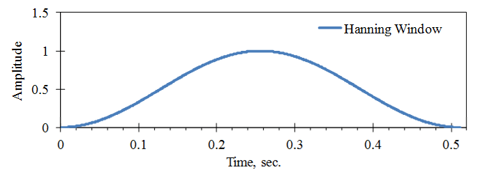
Figure 2.20. Hanning window used for a digital sample with SR = 2000 samples/sec. and N = 1024.
Example
Applying the Hanning window to the sine waves in Figure 2.19 produces the results in Figure 2.21. We should note several things. First, the level of spurious noise that the FFT generated from the non-periodic signal is greatly reduced for frequency bands at some distance from the peak frequency (called remote band leakage).
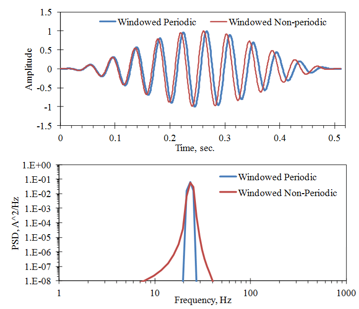
Figure 2.21. Effects of the Hanning window on the examples in Figure 2.19.
However, there is a trade-off. The PSD level is increased for the frequency bands adjacent to the peak frequency, even for the periodic signal. This is called sideband leakage. It also makes the frequency of the peak less certain. This is discussed further in the next lesson on frequency resolution.
Second, the PSD level at the peak frequency is reduced because the window reduced the mean-square amplitude of the signal in the time sample. This reduction can be corrected by dividing the PSD values by the mean square amplitude of the window function,  . This is 0.375 for the Hanning window and is usually included in the PSD computation. We can then revise Equation 3 to:
(2) 
(3) 
Equation 6
Leakage has also moved some of the peak value into the sidebands. This must be accounted for by using Equation 4 to sum the mean square values in the frequency bands around the peak instead of just using the peak value.
Learn more: Window Functions for Signal Processing