Normal (Gaussian) Distribution
March 29, 2018
Getting Started
Power Spectral Density
Converting Recorded Data
Statistics & Probabilities
Test Control
Back to: Random Testing
The normal, or “Gaussian,” distribution is an important probability function in statistical analysis. Another more recognizable name for it is the bell curve. Equation 9 defines the Gaussian probability density function (PDF) p(x).
(1) 
Equation 9
Figure 3.6 displays a normalized Gaussian PDF, where μ is the mean and σ is the standard deviation of the variable x. The mean value and standard deviation define the Gaussian distribution. The distribution is symmetrical, so its skewness equals 0, and kurtosis equals 3.
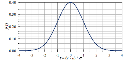
Figure 3.6. A normal (Gaussian) PDF; the “bell curve.”
Historical Background

Carl Friedrich Gauss, 1777 – 1855
German mathematician Carl Friedrich Gauss derived the Gaussian distribution’s basic form in his 1809 monogram on the motion of planets and comets.
Using the function e –kδ2 to represent the distribution of random errors (δ) in a measurement (where k is a scale factor), Gauss could prove that the least-squares method of fitting data generated the most probable result. He also used the distribution to statistically determine if the mean value of a series of measurements had this random error (visit the lesson on Confidence Intervals.)
Gaussian Distribution & Random Testing
Many statistical analyses assume a Gaussian distribution of data, including random vibration testing. The statistics of a random waveform define its distribution function. Most notably, the data set’s statistics define the first four central moments of the function: mean, variance, skewness, and kurtosis.
- Mean: The average acceleration value.
- Variance: The average of the squared difference from the mean.
- Skewness: The spread of acceleration values about the mean.
- Kurtosis: The deviation of acceleration peaks from the mean.
Modern vibration controllers assume the control signal has a Gaussian distribution, meaning the skewness is 0 and kurtosis is 3. This assumption can potentially lead to error if the waveform’s peak accelerations exceed ±3σ from the mean. However, for the purpose of this course, we can assume random vibration has a Gaussian distribution.
Cumulative Distribution Function (CDF)
The cumulative distribution function (CDF) is another probability distribution function. The CDF plots the probability that x is less than a set value X and is often written as P(x < X). Figure 3.7 displays the CDF for normal distribution.
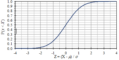
Figure 3.7. The normal cumulative distribution function.
Mathematically, it is given by Equation 10, where erf(…) is the error function.
(2) ![\begin{equation*} P(x<X)=\int_{-\infty}^{X}p(x)dx=\frac{1}{2}\left[1+\text{erf}\left(\frac{x-\mu}{\sqrt{2}\sigma}\right)\right] \end{equation*}](https://vru.vibrationresearch.com/wp-content/ql-cache/quicklatex.com-719eaa9870987e1bef821cb1fd67eba1_l3.png "Rendered by QuickLaTeX.com")
Equation 10
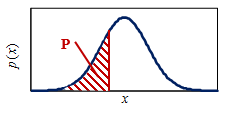
Graphically, the equation is represented by the area P in the following image. The total area under the PDF curve is equal to 1 by definition.
Probability Plots
Another way to plot the CDF is to convert the vertical axis scale, which produces a straight line for normal distribution. The result is called a normal probability plot. With this plot, it is easier to visually determine if data are normally distributed.
In the “old days” when things were plotted by hand on graph paper, there was a standard form called probability graph paper (Figure 3.8). As most computer graphing programs do not have this capability, a similar graph can be constructed by mapping the CDF values back to the normal Z values, then plotting these values versus the actual ones.
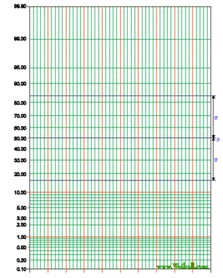
Figure 3.8. Probability graph paper.
Figure 3.9 is an example of normal probability plots using car vibration and turbulent pressure data from Figures 3.1 and 3.3. The straight diagonal line represents the normal distribution.
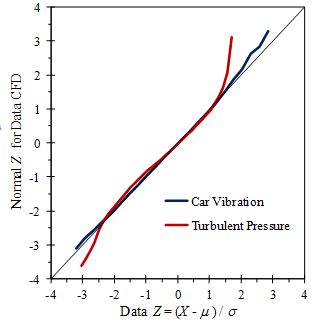
Figure 3.9. Normal probability plots of measured data from Figures 3.1 and 3.3.
The car vibration data closely follows the normal distribution, while the turbulent pressure data deviates significantly at the two ends of the distribution.