Probability Distributions Introduction

March 29, 2018

We cannot predict the amplitude of a random waveform at a specific time because it is non-deterministic, meaning it displays different characteristics for each test run. However, test engineers need to approximate vibration levels to avoid over or under-testing.

The probability distribution is a statistical method of determining the probability that a random waveform’s amplitude is within certain limits. A probability density function (PDF) is a histogram of a signal’s probable vibration distribution. The distribution is usually in a normalized form, displayed as the number of standard deviations from the mean. Test engineers can use a PDF to determine how likely the amplitude is to exceed some standard deviation (1σ, 3σ, etc.).

Computing a PDF

When a signal is digitized into a series of values (x_n, n = 1, …, N), the values become a sample set of the signal. An algorithm computes a probability histogram by categorizing the samples (m) into bins over the signal’s amplitude range. Figure 3.4 illustrates this process using the car vibration data from Figure 3.1.

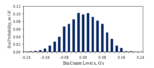
probability density function of car vibration

Figure 3.4. Histogram of the car vibration signal from Figure 3.1.

The plot displays the fraction of samples in each bin, m/N, versus the bin level as a bar chart, where the bin width (Δx) equals 0.02G. The sum of all the bins equals 1, but their amplitude range depends on the value of Δx.

To compute a PDF, the algorithm divides the fraction of samples in each bin by the bin’s width, Δx.

(1) $\begin{equation*} \text{PDF}=\frac{m}{(N\Delta{x})} \end{equation*}$

Figure 3.5a displays a PDF as a line graph. The PDF can be normalized further by plotting it over the number of standard deviations from the mean (Figure 3.5b).

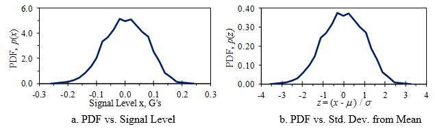
(2) $\begin{equation*} z=\frac{(x-\mu)}{\sigma} \end{equation*}$

sample probability density functions (PDF)

Figure 3.5. Sample PDFs of the vibration signal from Figure 3.1.

These are called sample PDFs. The true PDF is found in the limit as N approaches infinity and the number of bins approaches infinity (with the bin sizes becoming infinitesimal). In either case, the area under the PDF curve is 1.

PDF and Random Vibration

The following lessons examine the PDF for ideal statistical distributions. For these distributions, we can describe the PDF as a continuous function of the amplitude, x. It plays a significant role in understanding random vibration analysis.