Central Limit Theorem

March 29, 2018

The central limit theorem states that the sum (or average) of multiple sets of N random variables will move toward a normal distribution as N increases. The French mathematician Laplace proved this theorem for a number of general cases in 1810 [2].

Laplace also derived an expression for the standard deviation of the average of a set of random numbers. This expression confirmed what Gauss assumed for his derivation of the normal distribution.

Examples of the Central Limit Theorem

The simplest and most remarkable example of the central limit theorem is the coin toss. If a “true” coin is flipped N times, the probability of q heads occurring is given by the binomial distribution (Equation 11).

(1) $\begin{equation*} P(q)=\frac{N!}{2^N(N-q)!q!} \end{equation*}$

Equation 11

Figure 3.10 is a histogram of the binomial distribution compared to the normal distribution for 6 coin tosses. There is good agreement between the two distributions, even with only 6 tosses. However, the tails of the normal distribution extend beyond the possible q values.

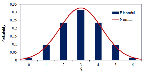
Figure 3.10. Probability of q heads for 6 coin tosses.

In 1733, the French mathematician De Moivre noticed this agreement between distributions. He used the following equation as an approximation for the cumbersome calculation for a large N value. However, he did not generalize it to other cases.

(2) $\begin{equation*} \left(\frac{2}{\pi N}\right)^{1/2}e^{-(2/N)(q-2/2)^2} \end{equation*}$

Averaging a Random Variable

Another example is the average of a random variable x that is uniformly distributed between -0.5 and 0.5. This distribution could be the range of uncertainty in measurement. There is a gradual convergence to the normal distribution as more random variables are added to the average (Figure 3.11).

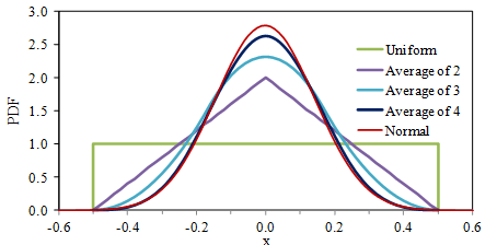
Figure 3.11. PDF of the averages of uniformly distributed random variables.

When the PDF‘s magnitude is on a linear scale, it is not clear what is happening at the distribution tails. This lack of clarity can be corrected by plotting the magnitude on a logarithmic scale. In doing so, the large deviation between the average of four uniformly distributed random variables and the normal distribution is visible at the distributions’ tails. This deviation is significant in cases where a signal’s extreme values are critical to understanding a product’s behavior, such as in fatigue analysis.