Calculating PSD from a Time-history File
June 25, 2019
Getting Started
Power Spectral Density
Converting Recorded Data
Statistics & Probabilities
Test Control
Back to: Random Testing
Vibration Research software uses Welch’s method for estimating the power spectral density (PSD). This method applies the fast Fourier transform (FFT) algorithm to its estimation of power spectra.
In regards to his method, Peter D. Welch said, “[the] principal advantages of this method are a reduction in the number of computations and in required core storage, and convenient application in nonstationarity tests.”1
Many programs implement Welch’s method is because the FFT makes it computationally efficient.2 The process begins with Gaussian-distributed time-domain input data—i.e., a time-history file.
Summary: Calculating PSD Using the FFT
- Partition data into frames of equal length in time
- Transform each frame into the frequency domain using the FFT
- Convert frequency-domain data to power by taking the squared magnitude (power value) of each frequency point
- Average the squared magnitudes of each frame
- Divide the average by the sample rate to normalize the PSD to a single hertz (Hz) bandwidth
A few additional factors affect the final PSD, including windowing and overlapping. Let’s look at each step in more detail.
Moving to the Frequency Domain
Figure 2.8 shows five seconds of Gaussian-distributed random vibration data in a time-history file. The peak acceleration appears to be around -30 G.
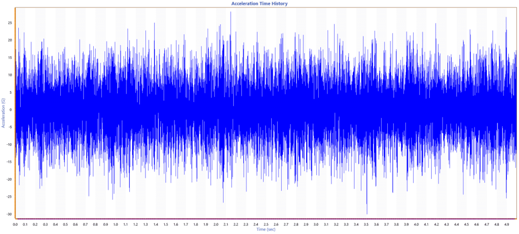
Figure 2.8. A five-second time-history graph.
For a different perspective of the vibration data, we can view it in the frequency domain. Moving to the frequency domain requires two calculations: the FFT and PSD.
Fast Fourier Transform (FFT)
The FFT transforms time-domain data into the frequency domain. This transformation itself does not inherently involve windowing, averaging, or normalization—it simply converts the data into its frequency components.
While engineers often use FFT graphs to monitor the frequency spectrum, such as observing changes in frequency content in real time or analyzing a time-history file, the FFT alone does not provide information about energy distribution.
To analyze energy distribution across the frequency spectrum, we calculate the power spectral density (PSD) from the FFT. The PSD quantifies how energy is distributed over frequency, offering a clearer understanding of the signal’s power content. This makes the PSD a commonly-used tool for vibration testing, where energy distribution across frequencies impacts system behavior and performance.
Calculating the PSD from a Time-history File
The steps to calculating PSD are as follows:
1. Divide the time-history file into frames of equal time length
First, the time-history file is divided into frames of equal time length. The lines of resolution and sample rate determine the width of each frame. There are two samples per analysis line.
In Figure 2.9, the recorded time history was sampled at 8,192 Hz and 4,096 lines of resolution. The resulting frame width was one second. If the lines of resolution value was 1,024, the frame width would be 0.25 seconds.
Using a sample rate that is an exponential of 2 (2n) usually results in a PSD with lines spaced at a convenient interval. This is important to remember when selecting an initial sample rate.
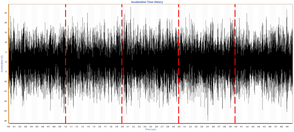
Figure 2.9. A time-history graph divided into equal frames.
Note: for more information on adjusting lines of resolution, consider reviewing the following resource: Adjusting Random Lines of Resolution technical note.
2. Calculate the FTT for each frame after applying a window function
The FFT regards data as an infinite series, interpreting each frames’ starting and ending points as though they are adjacent. However, random data are not an infinite series, so a window function must be applied to each frame before calculating its FFT.
Without a window function, differences between the starting and ending points of a frame can create a sharp transition or discontinuity. These discontinuities produce transient spikes that appear as high-frequency energy in the FFT, leading to a phenomenon known as spectral leakage.
Spectral leakage affects the accuracy of the FFT calculation by amplifying the impact of the discontinuities. Applying a window function reduces the emphasis on these transitions, minimizing spectral leakage and improving the FFT’s representation of the data.
Ideally, the starting and ending points of each frame would align perfectly. Since this is rarely the case with real-world data, window functions are necessary to minimize discontinuities and their effects on the spectral analysis (Figure 2.10).
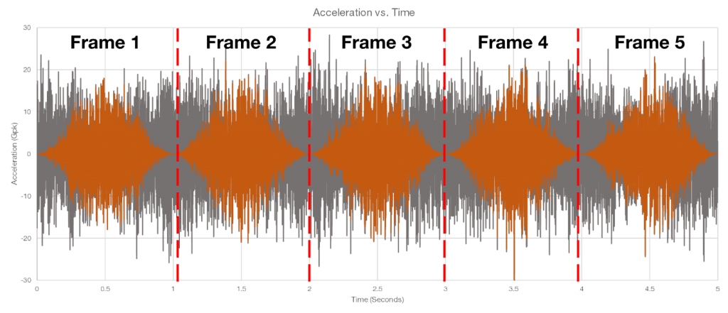
Figure 2.10. Applying a window function on each frame to reduce spectral leakage.
Windowing
There are multiple window functions. Selecting the most suitable one depends on the application. A window function is evaluated by two key components:
- Side lobe: Impacts leakage in the frequency domain
- Main lobe: Affects frequency resolution
Figure 2.10 illustrates a Hanning window function. The grey waveform is the original waveform, and the orange waveform is the windowed data.
Key characteristics of the Hanning window:
- High and wide main lobe
- Side lobes at nearly zero
- Minimal discontinuity between the starting and ending points, resulting in accurate frequency measurements
The Hanning and Blackman window functions are most common in vibration testing. Both functions have a good frequency resolution, minimal discontinuity, and, therefore, minimal leakage. Other window functions may be appropriate for other applications.
For a comprehensive list of common (and not-so-common) window functions, view the Table of Window Functions Details.
Calculating the FFT for Each Frame
An FFT is calculated for each frame using the windowed data, thereby transforming the signal from the time domain into the frequency domain (see Figure 2.11.) This linear transformation gives us the ability to observe the frequency content of the time-history waveform.
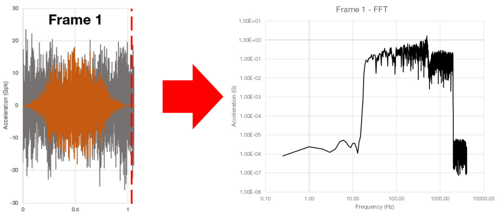
Figure 2.11. Calculating the FFT for each frame.
3. Square the individual FFTs for each frame and find an average
Next, square the individual FFTs for each frame and find the average squared amplitude (Figure 2.12).
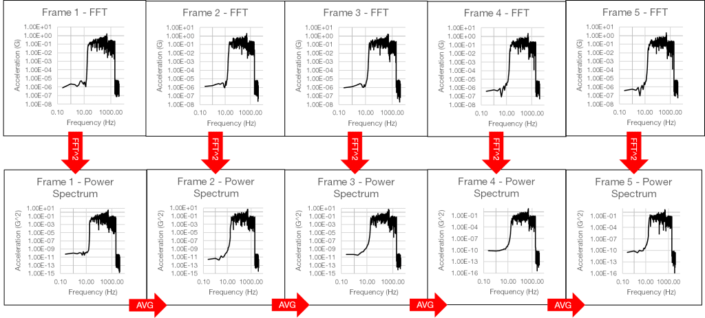
Figure 2.12. Squaring the individual FFT and finding the average squared amplitude.
The PSD displays the average energy at a single frequency over a period of time. Initially, it will have a variance or “hashiness.” As the average collects more frames of similar data, the overall variance will decrease, the accuracy will increase, and the PSD will appear much smoother.
The total amount of time included in a PSD is related to the averaging parameter called degrees-of-freedom (DOF). The more frames of data that are averaged together, the higher the DOF.
Simply put, more FFTs will result in a better PSD. However, large numbers of FFTs require more time to collect and calculate.
Note: for more information on degrees of freedom, consider reviewing the following resources:
4. Normalize the calculation to a single hertz
Finally, the algorithm takes the average squared FFT and normalizes it to a single hertz, and a PSD is determined (Figure 2.13). For acceleration, the resulting unit is G2/Hz.
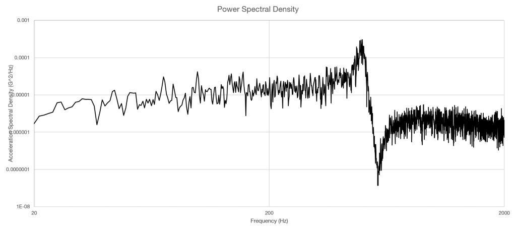
Figure 2.13. The resulting power spectral density (PSD).
Using the PSD, the response of the device under test is clear. As more frames of data are added to the PSD, the variance will continue to decrease and the PSD will become smoother.
For a more in-depth look at variance and methods of PSD smoothing, watch the video on Instant Degrees of Freedom. iDOF® is a feature from Vibration Research that quickly and effectively reduces the variance and creates a smooth PSD. This is the only mathematically justified method for displaying a smooth PSD trace in a short period of time.
Additional Parameters to Consider
Overlapping
Overlapping is an additional technique that engineers often use during PSD calculation, although it is not required. It includes more of the original data in the PSD and generates more degrees of freedom within a defined period.
With a 0% overlap, each frame of data is completely separated. When frames are overlapped, some data in each frame are not accounted for due to the applied window functions. For each frame of data in the PSD, two degrees of freedom are calculated for the total average.
Example
If we create a PSD with:
- 0% overlap
- 120 DOF
- 8,192 Hz sample rate
- 4,096 lines of resolution
- Hanning window function (1-second frames)
We will need to average 60 seconds worth of data to achieve 120 degrees of freedom.
With a 50% overlap, there would be 0.5 seconds between the start of each frame, but each frame would still be 1 second in length. Frames do not result in 2 DOF per FFT when they are overlapped. A 50% overlap would result in around 1.85 DOF per FFT; a 75% overlap would result in around 1.2 DOF per FFT.
Therefore, for a 50% overlap, 120 DOF, 8,192Hz, 4,096 lines of resolution, and a Hanning window PSD, we can achieve the desired PSD in 64.8 frames in 32.4 seconds.
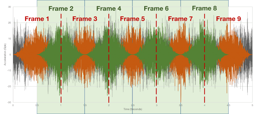
Figure 2.14. Overlapping windowed frames.
In the original example with 0% overlap, there were five frames of data, resulting in 5 FFTs. With the 50% overlap shown in Figure 2.14, the same section of data results in 9 FFTs.
Lines of Resolution
The last parameter to consider in the PSD calculation is the lines of resolution. Along with the sample rate, the lines of resolution value determines how far apart each analysis point is spaced on the PSD. A higher value will result in a more accurate PSD but requires a larger number of samples.
Many test standards require a specific lines of resolution value for a resonance to properly display the peak. If too few lines are used in a PSD, the result is similar to under-sampling a waveform: the distance between analysis points will be too great and the gap between will not be appropriately accounted for. A minimum requirement of three or more lines of resolution is needed to properly resolve a resonance.