The FFT and Digital Sampling

March 29, 2018

The fast Fourier transform (FFT) is a computer algorithm developed by James Cooley and John Tukey.¹ The algorithm computes the coefficients for the Fourier series that represents a sequence.

(1) $\begin{equation*} x(t) = \bar{x} + \sum_{i=1}^{\infty}{[C_{i}\cos(2 \pi f_{i} t)} + S_{i}\sin(2 \pi f_{i} t)]} \end{equation*}$

Equation 1

The number of samples (N) in the FFT must be an integer power of 2. Therefore, N = 2^p, where p is a positive integer. This rule minimizes the number of multiplications—and therefore the computation time—needed to compute the coefficients of the Fourier series.

The Fourier series represents a time signal x(t) by the sum of cosine and sine waves where x̅ is the mean value. In theory, this sum has an infinite number of terms. In practice, it is limited by the sample rate. The usable frequencies in the FFT are limited to those less than one-half of the sample rate. The Nyquist frequency ( f_q) represents half the sampling rate of a system.

Digital Sampling and Potential Discontinuity

The number of samples is often denoted by N = 1k, 2k, 4k, and so on, where k = 1024. It is customary to number the samples starting with 0, so the samples are labeled x_n, n = 0, … , 7.

For example, consider the point sample N = 8 in Figure 2.15. The samples are spaced in time by Δt = 0.5 msec, so SR = 1 / Δt = 2000 samples/sec.

The total time duration of this digital sample is T = N *Δt = 4.0 msec. However, there is no sample at T = 4.0 msec because the N samples are assumed to start at t = 0. The Fourier series assumes the signal is periodic in time T, so the sample at T would, by definition, be the same value as the first sample (illustrated by the dashed point in Figure 2.15).

As this is not the case for an arbitrary random signal, a potential error is introduced. The discontinuity between the end of the digitized signal and the beginning of the presumed periodic repetition is covered in the Windowing lesson.

The usable frequencies in this example are shown in Figure 2.16, where the FFT determines the amplitude coefficients C_i and S_i. The sum of all the cosine and sine waves with their determined coefficients results in an exact duplicate of the signal at the sampled points.

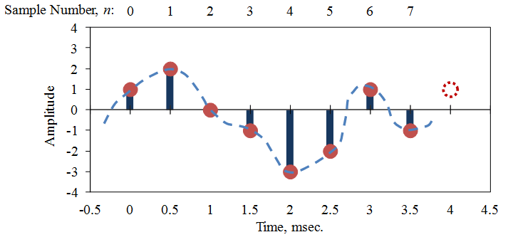
Figure 2.15. A digitally sampled time signal, where the digital sample is denoted by red dots and x(t) by a blue dashed line.

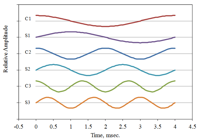
Figure 2.16. A set of cosine and sine waves used to represent the signal in Figure 2.15.

Determining the Fourier Series Coefficients

Each Fourier coefficient is determined by multiplying Equation 1 by the associated cosine or sine wave. Then, the average value of these products over N samples is computed. The result is equation 2, where f_j = j / T, j = 1, …, N/2 – 1.

(2) $\begin{equation*} \frac{1}{N} \sum_{n=0}^{N-1}{[C_{i}\cos(2 \pi f_{j} t_{n}) * x_{n}]} = \frac{1}{2}C_{j} \end{equation*}$

(3) $\begin{equation*} \frac{1}{N} \sum_{n=0}^{N-1}{[S_{i}\sin(2 \pi f_{j} t_{n}) * x_{n}]} = \frac{1}{2}S_{j} \end{equation*}$

Equation 2

The right side of Equation 2 is the simplified version. The average value of the product of two different cosine/sine waves is zero; the average value of the product of a cosine/sine wave with itself is one-half. This simplification assumes the averages are collected over an integer number of cycles, which is the case for the FFT.

The left side of Equation 2 requires many multiplications to complete. In the FFT algorithm, N is an integer power of 2 and many of these computations are redundant. More information on the details of the FFT computation algorithm is in reference.²

Computing Fourier Series Coefficients with Long-Form Equation

Continuing with the computation of the Fourier series coefficients using the long hand version of Equation 2 gives:

(4) $\begin{equation*} x(t)=x0, x1, x2, x3, x4, x5, x6, x7 = 1, 2, 0, -1, -3, -2, 1, -1 \end{equation*}$

(5) $\begin{equation*} \bar{x}=(x0 + x1 + x2 + x3 + x4 + x5 + x6 + x7)/N = -0.375 \end{equation*}$

(computed as C₀ at f₀ = 0 in the FFT)

(6) $\begin{equation*} C_{1}=\frac{2}{N}(x0+\sqrt{2}x1-\sqrt{2}x3-x4-\sqrt{2}x5+\sqrt{2}x7)=1.707; f_{1}=\frac{1}{T}=250Hz \end{equation*}$

(7) $\begin{equation*} S_{1}=\frac{2}{N}(\sqrt{2}x1+x2+\sqrt{2}x3-\sqrt{2}x5-x6-\sqrt{2}x7)=-0.457 \end{equation*}$

(8) $\begin{equation*} C_{2}=\frac{2}{N}(x0-x2+x4-x6)=-0.75; f_{2}=\frac{2}{T}=500Hz \end{equation*}$

(9) $\begin{equation*} S_{2}=\frac{2}{N}(x1-x3+x5-x7)=-0.5 \end{equation*}$

(10) $\begin{equation*} C_{3}=\frac{2}{N}(x0-\sqrt{2}x1+\sqrt{2}x3-x4+\sqrt{2}x5-\sqrt{2}x7)=0.293; f_{3}=\frac{3}{T}=750Hz \end{equation*}$

(11) $\begin{equation*} S_{3}=\frac{2}{N}(\sqrt{2}x1-x2+\sqrt{2}x3-\sqrt{2}x5+x6-\sqrt{2}x7)=0.957 \end{equation*}$

These computations illustrate the redundancy in the calculations. Note that some FFT algorithms (such as those in Excel) do not multiply by 2/N in their computations. Instead, they only return the summation values in Equation 2.

Computing the PSD of the signal

The values of the PSD are the mean square amplitudes of the FFT at each frequency divided by the frequency spacing, Δf = 1 / T (Eq. 3). The value at f₀ = 0 is computed differently because it represents the mean value given by C₀ (since cos(0) = 1).

(12) $\begin{equation*} PSD_{x}(0) = \frac {C_{0}^2}{\Delta f} \end{equation*}$

(13) $\begin{equation*} PSD_{x}(f_{j}) = \frac {0.5(C_{j}^2 + S_{j}^2)}{\Delta f}; j=1, \dots, N/2-1 \end{equation*}$

Equation 3

Figure 2.17 displays the PSD for Figure 2.15, where A represents units x. Each PSD value is associated with a frequency band centered at the associated FFT frequency. The frequency bandwidths are equal to Δf (except for f = 0, where the bandwidth is Δf / 2).

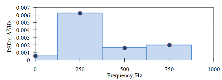
Figure 2.17. The PSD of the signal in Figure 2.15.

The FFT computes values for N frequencies, f_j = j /T, j = 0, …, N–1, but the PSD only requires the first N/2 values. Additionally, the signal x(t) necessitates a low-pass filter before digital sampling to ensure there is no frequency content above the Nyquist frequency. Otherwise, errors will occur in the FFT computation. This idea is discussed further in the Aliasing lesson.

Recovering the Mean Square, Standard Deviation, and RMS

The mean square, standard deviation, and RMS values of the time signal can be (approximately) recovered from the PSD. The PSD is the mean square value of the Fourier series components. Therefore, the mean square of the signal is found by summing the PSD values and multiplying by the frequency bandwidth, Δf = 1 / T , (Eq. 4).

(14) $\begin{equation*} \bar{x^2} = \Delta f * \sum_{j=0}^{N/2-1} PSD_{x}(f_{j}) \end{equation*}$

Equation 4

The RMS value is given by the root mean square of x.

(15) $\begin{equation*} x_{rms} = \sqrt{\frac{1}{n}(x_{1}^2 + x_{2}^2,\dots , + x_{n}^2)} \end{equation*}$

The standard deviation is given by:

(16) $\begin{equation*} \sigma = \sqrt{\bar{x^2} - (\bar{x})^2} \end{equation*}$

Table 1 compares the values computed from the signal in Figure 2.15 and the PSD in Figure 2.17. There are small differences because the FFT uses the presumed signal value at T, whereas the calculation from the signal samples does not. This is discussed further in the Windowing lesson.

Table 1. Comparison of the values computed from the signal and the PSD.

	Using x_n	Using PSD
Mean Square Value, x̅2̅	2.625	2.609
Mean Square Value, x̅	– 0.375	– 0.375
Standard Deviation, σ	1.576	1.571

Note: In many random vibration signals, the mean value is assumed to be zero, so x_rms = σ. This is not the case in this example.