Regression Analysis and Least Squares

March 29, 2018

In non-mathematical terminology, regression analysis involves fitting smooth curves to scattered data. Around 1800, determining the best method for regression analysis of the planets’ orbits was a major motivating factor for the development of the normal distribution [1], the central limit theorem [2], and the method of least squares [5]. Regression analysis is relevant today for important data such as global surface temperature (Figure 3.17).

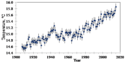
Figure 3.17. Linear regression of global surface temperatures.

In its simplest form, linear regression fits a straight line to a series of data points (x_n, y_n), n = 1, …, N, as Figure 3.17 illustrates. The equation for the line is y = ax + b, and we determine a and b. The error, or residual, is the difference between the line and data points at each x_n: e_n = y_n – ax_n – b.

The Least Squares Method

The method of least squares determines the “best” values for a and b. This is achieved by summing the squares of the residuals, e_n, and finding the values of a and b that minimize the sum. Using calculus, the derivatives of the sum are set to zero with respect to a and b. Then, the two equations are solved for a and b. Equation 19 is the resulting formula:

(1) $\begin{equation*} a=\frac{\sum_{n-1}^{N}(x_{n}-\bar{x})(y_{n}-\bar{y})}{\sum_{n-1}^{N}(x_{n}-\bar{x})^2}; b=\bar{y}-a\bar{x} \end{equation*}$

(2) $\begin{equation*} \text{where the mean values are }\bar{x}=\frac{1}{N}\sum_{n=1}^{N}x_{n}\text{ and }\bar{y}=\frac{1}{N}\sum_{n=1}^{N}y_{n} \end{equation*}$

Equation 19

To obtain the confidence interval for the curve fit, we can assume the errors are normally distributed. Equation 20 calculates the variance of the residuals. N – 2 is in the denominator because the two equations for a and b reduced the degrees of freedom by 2.

(3) $\begin{equation*} \sigma_{\varepsilon}^2=\frac{1}{N-2}\sum_{n=1}^{N}\varepsilon_{n}^2 \end{equation*}$

Equation 20

Now, we must add the variance of the determination of the y_n data, σ_yn². It is often assumed that the error bound for measurement is equal to 2σ_y based on a 95% confidence level. The standard deviation for the line values, y, is:

(4) $\begin{equation*} \sigma_{y}=\sqrt{\sigma_{\varepsilon}^2+\sigma_{y_{n}}^2} \end{equation*}$

Equation 21

The R-squared coefficient is a common measurement to determine the best fit for the regression analysis (Equation 22).

(5) $\begin{equation*} R^2=1-\frac{\sum_{n=1}^{N}\varepsilon_{n}^2}{\sum_{n=1}^{N}(y_{n}-\bar{y})^2} \end{equation*}$

Equation 22

The square root of R² is often called the correlation coefficient, $r=\sqrt{R^2}$ . In the example of global surface temperatures (Figure 3.17), σ_e = 0.133º C. The error bound for each temperature measurement is ±0.1º C, so it is assumed that σ_yn= 0.050º C. Then, σ_y = 0.14º C, and the 95% confidence interval is ±0.28º C. The calculated value for R-squared is 0.83.

Using Log Values for Linear Regression

In many cases, data on a linear scale does not fit a straight line. Instead of a non-linear curve, it is convenient to use logarithmic values for the linear regression. For example:

log(y) vs. x
y vs. log(x)
log(y) vs. log(x)

Example

The damping in a structure causes the vibration to decay at the theoretical rate of A(t) = A_o e^-2π^{f ζ t}after impact. f is the frequency in Hz, t is the time in sec., and ^ζ is the critical damping ratio.

To determine the damping value, the RMS acceleration level is measured versus time after impact (see Figure 3.18a for f = 200Hz.)

The theoretical decay will be a straight line when plotted as log(A) = log(A_o) – [2π f ^ζ log(e)] t (Figure 3.18b). In this example, the linear regression equates the slope at -8.28, so ^ζ = 8.28 / [2π f log(e)] = 0.015.

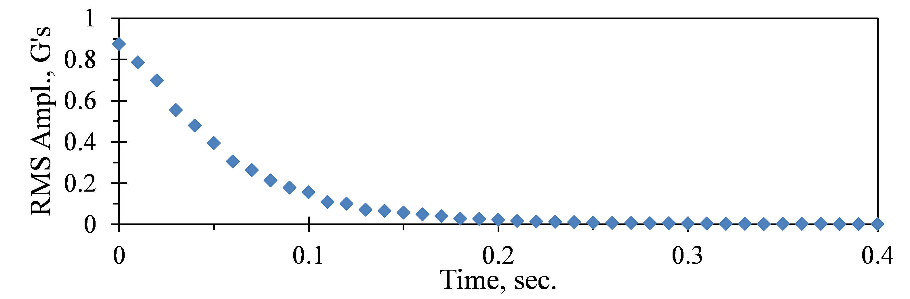
Figure 3.18a. RMS acceleration level measured vs. time after the structure is impacted for f = 200Hz.

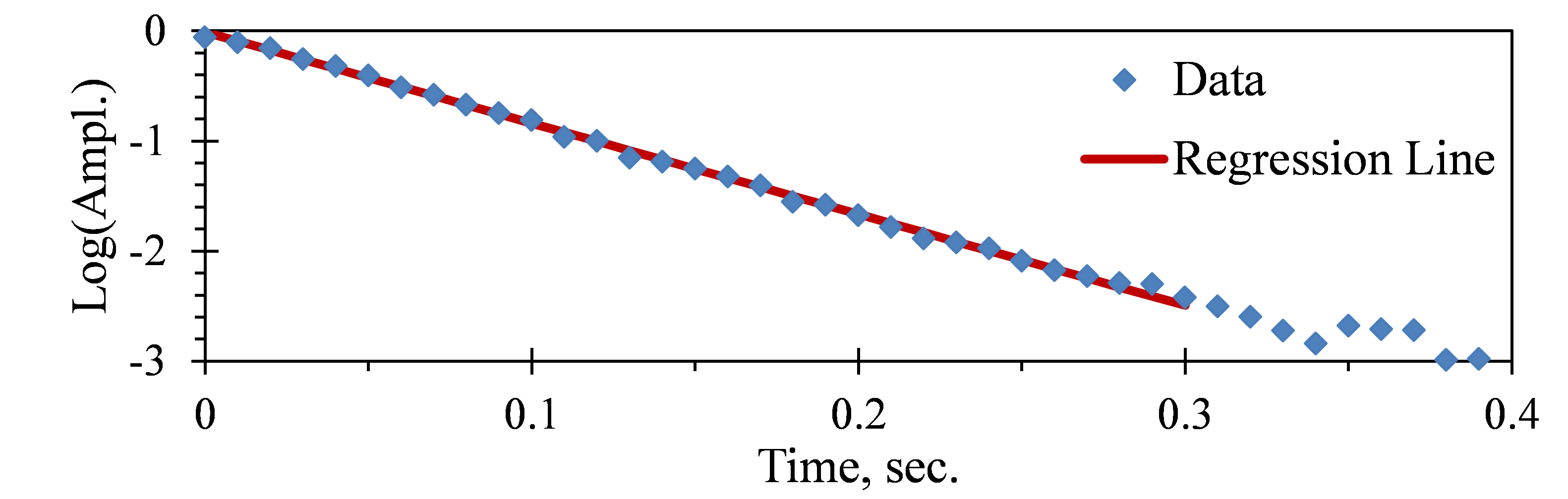
Figure 3.18b. Regression analysis of transient vibration decay.