Sampling at the Nyquist Rate
August 1, 2019
Sampling
Frequency Domain Consequences of Sampling
Reconstruction Via Interpolation
Quantization noise and over-sampling
Differential Quantization / Delta Modulation
Noise Shaping / Delta-Sigma Modulation
Back to: Sampling & Reconstruction
In Example 1, the time waveform x(t) was sampled at 𝖥s = 4 × 𝖿h. The resulting DTFT spectral images were spread out in the DTFT frequency domain.
By examining these results, it is apparent that the minimum sample rate is 𝖥s = 2 × 𝖿h. Anything less would result in the overlap of spectral images.
The 𝖥s = 2 × 𝖿h rate is called the Nyquist rate. Example 5 is similar to Example 4, but the sample rate 𝖥s is reduced to the Nyquist rate.
Frequency Content of a Waveform Sampled at Nyquist Rate (Ex. 5)
Given the time waveform illustrated in Figure 2.1:
(1) ![\begin{equation*} x(t)=\frac{1}{\sqrt{2\pi}}\left[\frac{\sin(t/2)}{t/2}\right]^2 \triangleq \frac{1}{\sqrt{2\pi}}sinc^2\left(\frac{t}{2}\right) \end{equation*}](https://vru.vibrationresearch.com/wp-content/ql-cache/quicklatex.com-c87be8fc3ce4df4c31c27b000c5246b5_l3.png "Rendered by QuickLaTeX.com")
The Fourier transform 𝖷̃(𝜔) is the triangle function illustrated in Figure 2.3 with the highest frequency component of 𝖿h = 1/2𝜋 Hz.
The waveform x(t) sampled at 𝖥s ≜ 2 × 𝖿h = 4 × 1/2𝜋 = 1/𝜋 gives a sample period of 𝜏 = 1/𝖥s = 𝜋 and is illustrated in Figure 2.5.
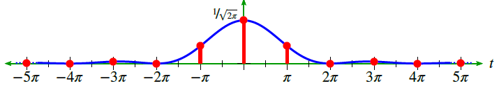
Figure 2.5. Sample sequence.
Using this sample rate and Theorem 1, a DTFT 𝖸̃(𝜔) of y(n) is expressed as:
(2) ![\begin{equation*} \tilde{Y}(\omega)=\sqrt{2\pi}F_{s}\sum_{n\in\mathbb{Z}}\tilde{X}(F_{s}[\omega-2\pi n]) \end{equation*}](https://vru.vibrationresearch.com/wp-content/ql-cache/quicklatex.com-0b03cc834fc4cacc1167504e5167328a_l3.png "Rendered by QuickLaTeX.com")
(3) ![\begin{equation*} =\frac{\sqrt{2\pi}}{\pi}\sum_{n\in\mathbb{Z}}\tilde{X}\left(\frac{1}{\pi}[\omega-2\pi n]\right) \end{equation*}](https://vru.vibrationresearch.com/wp-content/ql-cache/quicklatex.com-e78191df6d795edbbe6edb355b743672_l3.png "Rendered by QuickLaTeX.com")
Conclusion
- 𝖷̃(𝜔) repeats every 2𝜋 (this is true of all DTFTs)
- 𝖷̃(𝜔) reaches 0 when (1/𝜋) 𝜔 = 1 or 𝜔 = 𝜋
- The height of each triangle is
 or about 0.798 (see Figures 2.6 and 2.7)
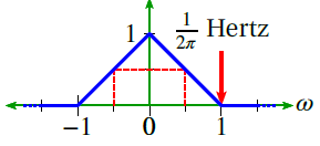
Figure 2.6. Fourier transform.
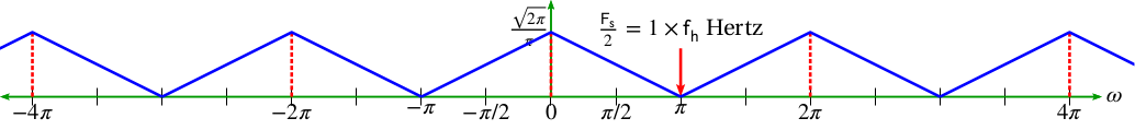
Figure 2.7. DTFT.