DTFT of a Sampled Sequence

July 24, 2019

Suppose there is a signal x(t) with a Fourier transform of $\tilde{X}(\omega)$ . The signal is sampled every 𝜏 seconds, yielding the sequence y(n) = x(n𝜏). From the sampled sequence, a calculation yields the discrete-time Fourier transform (DTFT) $\tilde{Y}(\omega)$ of y(n).

Both a Fourier transform $\tilde{X}(\omega)$ and a DTFT $\tilde{Y}(\omega)$ have been identified. They come from two different transform definitions but originated from the same signal, x(t).

This prompts the question: do $\tilde{X}(\omega)$ and $\tilde{Y}(\omega)$ look anything alike? The answer is yes; in fact, $\tilde{Y}(\omega)$ looks like a scaled and repeated version of $\tilde{X}(\omega)$ . Below, Theorem 1 and Example 1 offer a more precise description as to why this is.

Theorem 1

Defining the DTFT of a sampled sequence in terms of the Fourier transform of the sampled waveform.

Let 𝗒(𝑛) ≜ 𝗑(𝑛𝜏) be the sample sequence of a waveform 𝗑(𝑡). 𝖥_s = 1/𝜏 is the sample rate. Let 𝖸̆(𝜔) be the DTFT of 𝗒(𝑛) and 𝖷̃ (𝜔) be the Fourier transform of 𝗑(𝑡). Then:

(1) $\begin{equation*} \tilde{Y}(\omega)=\sqrt{2\pi}F_{s}\sum_{n\in\mathbb{Z}}\tilde{X}(F_{s}[\omega-2\pi n]) \end{equation*}$

Proof

This theorem is difficult to prove without resorting to an “engineering hack” methodology such as multiplying the waveform by a train of impulse functions. However, the proof is manageable when we leverage the somewhat obscure yet powerful inverse Poisson summation formula (IPSF).

(2) $\begin{equation} \tilde{Y}(\omega)\triangleq\sum_{n\in\mathbb{Z}}y(n)e^{-i\omega n} \end{equation}$	by definition of DTFT
(3) $\begin{equation} =\sum_{n\in\mathbb{Z}}x(n\tau)e^{-i\omega n} \end{equation}$	by definition of y(n)
(4) $\begin{equation} =\sum_{n\in\mathbb{Z}}x(n\tau)e^{-i\frac{\omega}{\tau}n\tau} \end{equation}$	because τ/τ = 1
(5) $\begin{equation} =\frac{\sqrt{2\pi}}{\tau}\sum_{n\in\mathbb{Z}}\tilde{X}\left(\frac{\omega}{\tau}+\frac{2\pi}{\tau}n\right) \end{equation}$	by IPSF
(6) $\begin{equation} =\sqrt{2\pi}\text{F}_{s}\sum_{n\in\mathbb{Z}}\tilde{X}(\text{F}_{s}[\omega-2\pi n])\text{ by }\text{F}_{s}=1/\tau \end{equation}$	and absolute summability

The DTFT of the sample sequence is the Fourier transform of the original waveform. It is:

Repeated every 2𝜋 radians (in discrete world frequency, which is every 2 × 𝖥_s Hz in real-world frequency)
Dilated (made narrower) by a factor of 𝖥_s
Scaled (made taller) by a factor of √2𝜋𝖥_s

Figures 2.1-2.4 illustrate the extraction of the frequency content of a sampled waveform with a sample rate of Fs = 4 x fh.

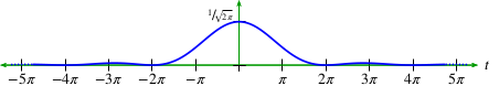
Figure 2.1. Time waveform x(t).

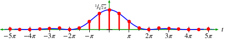
Figure 2.2. Sample sequence.

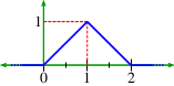
Figure 2.3. Fourier transform.

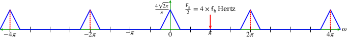
Figure 2.4. DTFT of y(n).

Examples 4 through 7 in this lesson and those that follow illustrate the importance of Theorem 1.

Frequency Content of a Sampled Waveform (Ex. 4)

F_s = 4 x f_h

Given the time waveform illustrated in Figure 2.1:

(7) $\begin{equation*} x(t)=\frac{1}{\sqrt2\pi}\left[\frac{sin(t/2)}{t/2}\right]^2 \triangleq \frac{1}{\sqrt2\pi}\text{sinc}^2\left(\frac{t}{2}\right) \end{equation*}$

The Fourier transform 𝖷̃ (𝜔) is the triangle function illustrated in Figure 2.3. The highest frequency component is 𝜔h = 1 radian/second or 𝖿h = 1/2𝜋 Hz. Therefore, the minimum sample rate is 𝖥s ≥ 2 × 𝖿h = 1/𝜋 and the maximum sample period is 𝜏 ≤ 𝖥_s = 𝜋.

The waveform 𝗑(𝑡) sampled at 𝖥_s ≜ 4 × 𝖿_h = 4 × 1/2𝜋 = 2/𝜋 (giving a sample period of 𝜏 = 1/𝖥_s = 𝜋/2) is illustrated in Figure 2.2.

With this sample rate and Theorem 1, the DTFT 𝖸̃(𝜔) of 𝗒(𝑛) is a repeated and scaled version of 𝖷̃ (𝜔). It is expressed as:

(8) $\begin{equation*} \tilde{Y}(\omega)=\sqrt{2\pi}F_{s}\sum_{n\in\mathbb{Z}}\tilde{X}(F_{s}[\omega-2\pi n]) \end{equation*}$

(9) $\begin{equation*} =\frac{2\sqrt{2\pi}}{\pi}\sum_{n\in\mathbb{Z}}\tilde{X}\left(\frac{2}{\pi}[\omega-2\pi n]\right) \end{equation*}$

Conclusion

𝖷̃ (𝜔) repeats every 2𝜋 (this is true of all DTFTs by definition)
𝖷̃ (𝜔) reaches zero when (2/𝜋) 𝜔 = 1 or 𝜔 = 𝜋/2; the higher the sample rate 𝖥_s, the narrower the triangle illustrated in Figure 2.3
The height of each triangle is $2\sqrt{2\pi}/\pi$ or about 1.596. The higher the sample rate 𝖥_s, the higher the triangle illustrated in Figure 2.3