Examples of Waveform Sampling

July 8, 2019

Typically, sampling involves taking measurements of a waveform at regular intervals and structuring these measurements as a sequence of values. The length of this interval is called the period and is often represented as 𝑇 or 𝜏 with the unit seconds. The rate 1/𝜏 is called the sample rate and is often denoted as 𝖥_s with the unit hertz (Hz).

The following is an example of sampling a cosine.

Sampling a Cosine (Ex. 1)

Suppose we have a waveform, w(t), that is a 100Hz cosine such that w(t) = cos(2𝜋100t).

Sampling at 𝖥_s = 4 x f_h = 400Hz (Figure 1.3) yields the sample sequence:

(1) $\begin{equation*} y(n)=(\!(… , -1, 0, 1, 0, -1, 0, 1, 0, -1, 0, 1, …)\!) \end{equation*}$

Similarly, sampling at 𝖥_s = 6 x f_h = 600Hz (Figure 1.3) yields the following sequence:

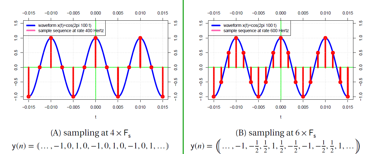
(2) $\begin{equation*} y(n)=(\!(… , -1, -\frac{1}{2} , \frac{1}{2} , 1, \frac{1}{2} , -\frac{1}{2} , -1, -\frac{1}{2} , \frac{1}{2} , 1, …)\!) \end{equation*}$

Figure 1.3. Sampling a cosine.

Although these two sequences are different, either can be used to perfectly reconstruct the original waveform w(t).

Retaining the Sample Rate

If a sampled signal is to be processed and eventually reconstructed, retaining the knowledge of the sample rate is extremely important. The concept of duration in time is lost without the knowledge of the sample rate during sampling, even though the time-ordering of the samples is preserved (e.g., y(1) occurred earlier in time than y(2)). Our second example further illustrates this point.

Sampling a Cosine without the Sample Rate (Ex. 2)

Suppose we have a waveform w1(t) that is a 1Hz cosine such that w1(t) ≜ cos(2𝜋t). Sampling at 4Hz (Figure 1.4) yields the sequence:

(3) $\begin{equation*} y_{1}(n)=(\!(..., -1, 0, 1, 0, -1, 0, 1, 0, -1, 0, 1,...)\!) \end{equation*}$

Similarly, a waveform w2(t) that is a 100Hz cosine such that w2(t) ≜ cos(2𝜋100t) sampled at 400Hz (Figure 1.4) yields the sequence:

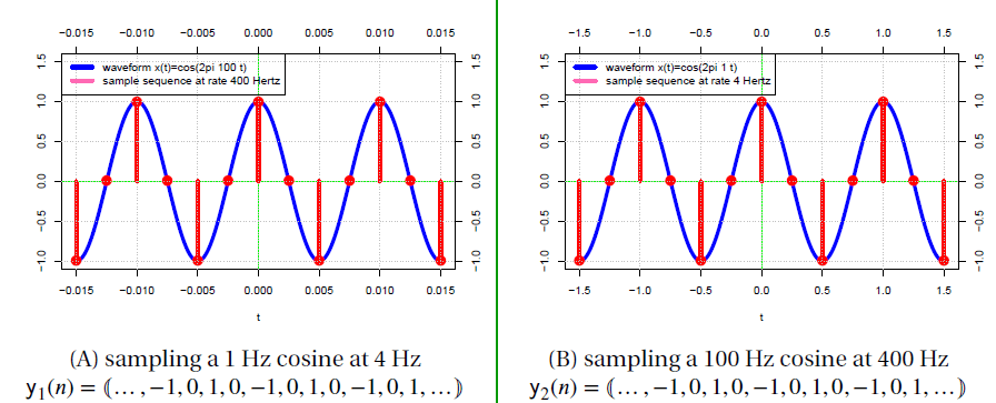
(4) $\begin{equation*} y_{2}(n)=(\!(..., -1, 0, 1, 0, -1, 0, 1, 0, -1, 0, 1,...)\!) \end{equation*}$

Figure 1.4. Sampling a 1 Hz cosine at 4 Hz and a 100 Hz cosine at 400 Hz.

The two sequences are identical (y1(n) = y2(n)) despite the fact that w1(t) is oscillating 100 times faster than w2(t) in real-time. Thus, we must know the value of the sample rate to properly reconstruct the waveform in the real world.