Displacement Conversion Validation
June 27, 2022
Back to: Getting to Know ObserVIEW 2022.1
Goal: To validate ObserVIEW’s displacement conversion and analyze the differences in a product’s displacement during a shock test.
Software: ObserVIEW, VibrationVIEW
Required licenses (ObserVIEW): Advanced
Required modules (VibrationVIEW): System Check, Shock
Introduction
This analysis sought to answer three questions:
- Does ObserVIEW’s dynamic displacement trace for a sensor at the shaker head match the expected displacement reported in the VibrationVIEW test profile during a shock test?
- How does the displacement differ between a sensor close to the shaker head to one further away?
- If there is a significant difference in displacement, does the sensor further from the shaker head experience higher or lower values?
Test Setup
The device under test was an aluminum cross. The center of the cross was attached to an electrodynamic shaker head, and a single-axis accelerometer was mounted at the top. A second, triaxial accelerometer was mounted to the end of one of the beams.
Both the sensors were piezoelectric accelerometers, which measure dynamic acceleration. In practical terms, they do not measure the constant pull of gravity but changes in acceleration. They report a voltage related to the movement of current to the connected devices.
The sensors were connected to a VR9500 and an ObserVR1000 portable data acquisition unit. The shaker was plugged into an amplifier to increase the controller’s output power. Additionally, the VR9500 COLA/Aux output was connected as an input on the ObserVR1000.
The VR9500 and ObserVR1000 were connected to a computer equipped with the VibrationVIEW 2022 and ObserVIEW 2022 software using Gigabit Ethernet cables.
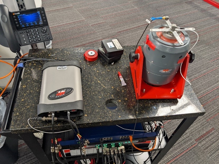
Figure 1. The shaker and ObserVR1000 on a portable cart and the VR9500 controller and amplifier on the first shelf.
VibrationVIEW Configuration
VibrationVIEW requires several steps before creating a test. First, select Configuration > Configure Hardware to connect to the VR9500 controller. This connection may prompt a program restart depending on the previous configuration.
Next, configure the inputs on the Configuration > Inputs dialog.
In the test setup, the triaxial accelerometer included TEDS information, but the single-axis sensor did not. The software read the sensitivity, unit, serial number, and calibration date for the triaxial sensor automatically, and the sensitivity information for the mount sensor (single axis) was provided by the manufacturer.
After verifying that the input information is correct, the configuration can be saved for later.
Finally, Accel Power was enabled for the sensors, which they required for measurement.
Select Apply after the inputs are set up.
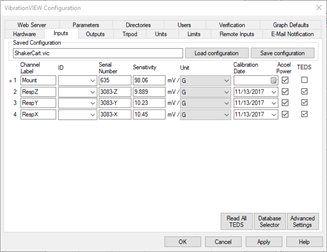
Figure 2. VibrationVIEW input configuration.
The VibrationVIEW test setup also requires shaker limits. On the Limits tab of the Configuration dialog, select the correct shaker model. If it is not on the list, the User Defined Limits option allows a manual entry of values.
We wanted the output voltage to be one of the inputs to the ObserVR1000, so the COLA/Aux output was set to Differential Output on the Outputs tab.
ObserVIEW Setup
In ObserVIEW, select File > Connect to Device > Configure Hardware and locate the ObserVR1000. Select Connect, and a Live Analyzer session will begin.
In the ObserVR1000 Settings pane, find the Inputs tab. The connected channels should be enabled and set up with most of the same settings as the VibrationVIEW configuration.
VibrationVIEW would provide acceleration power to the sensors, so accel power was not applied in ObserVIEW, and the voltage range was changed to 0-20V (see Figure 3.)
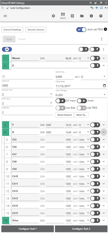
Figure 3. Example of an ObserVR1000 configuration.
System Check
A system check was performed in VibrationVIEW (recommended). The amplifier was turned on with minimal gain and a medium current limit. Then, a System Check test was selected from the VibrationVIEW Navigator.
The System Check test will run until a message appears, stating that the output voltage reached the safety threshold while input remained low.
Each time this notice appeared, the gain was increased, and the test was re-run. Eventually, a sine wave appeared on the acceleration waveform graph for channels Mount and RespZ. This waveform indicated that the system check was successful.
In ObserVIEW, the Mount, Z, and Drive channels matched the acceleration waveform. The drive may have had a phase shift applied to it due to unpredictable latencies in the system, which could be ignored.
Creating and Running the Shock Test
After the system was set up correctly, the test could be created and run.
To create a shock test in VibrationVIEW, select New Test > Shock.
Shorter pulse durations were desired, so the pulse width was set to 8ms. The peak amplitude was set to 30G.
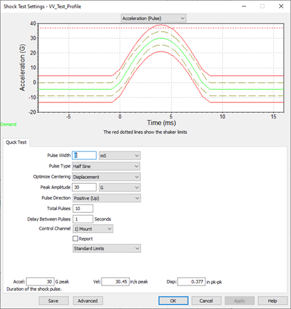
Figure 4. Shock test settings.
The test revealed that the required output voltage exceeded the test limit. Since it was not yet close to the system limit, it was increased by changing the Max output values under Starting drive limits and Running drive limits using Edit Test > Advanced > Limits. A value of 3V was all that was necessary in this case.
Note: If trying to determine the needed output voltage, create a Drive Output vs. Input Readings graph, run a test, and determine where the control and demand will meet.
Finally, start the test and watch the shock data stream into ObserVIEW.
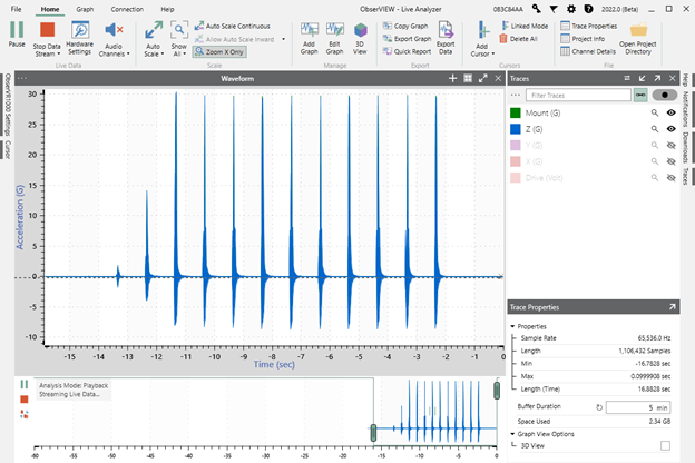
Figure 5. Shock data streaming into ObserVIEW from the ObserVR1000.
Analysis and Comparison
We zoomed in on one pulse of maximum amplitude and exported the selection range to a VFW file. This would allow for the displacement analysis of a single pulse without other pulses causing unexpected results.
We opened the exported VFW in ObserVIEW and added a displacement waveform. A corner frequency of 5Hz negated the low-frequency drift present in the accelerometer’s lower sensitivity data. The triaxial accelerometer could measure a greater range of amplitudes but had lower amplitude resolution. A max cursor and min cursor were also added to find the peak-to-peak amplitude change during the shock.
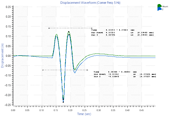
Figure 6. Cursors reveal minimum and maximum displacement.
The minimum values were subtracted from the maximum ones to provide a peak-to-peak value. It was computed by double integrating the acceleration data the ObserVR1000 measured. The results are recorded in the table below.
| Measurement | Maximum displacement (in) |
Minimum displacement (in) |
Peak-to-peak displacement (in) |
| Mount | 0.12312 | -0.22252 | 0.34564 |
| Response Z | 0.10795 | -0.23646 | 0.34441 |
The peak-to-peak measurement was slightly less than the 0.377 theoretical from VibrationVIEW. There are a couple of factors that could have contributed to this:
- The ObserVR1000 had a filter that removed extremely low-frequency content from the recordings.
- Due to the low sensitivity of the response accelerometer, the corner frequency had to be increased to 5Hz. This could have removed some of the lower frequency content, which could have contributed to the greater displacement.
Given the low sensitivity of the response accelerometer, we cannot confidently conclude whether it experienced higher or lower displacement. However, the displacement values reported by ObserVIEW are similar to the theoretical peak-to-peak displacement, providing confidence that ObserVIEW’s displacement conversion works well with shock acceleration data.