Convert Acceleration to Displacement
June 27, 2022
Back to: Getting to Know ObserVIEW 2022.1
Perform a unit conversion from acceleration to velocity or displacement on time graphs.
Example
Analyzing Long-term Car Strut Displacement
Goal: To determine a strut’s range of motion and its min/max displacement in the operational environment.
Software: ObserVIEW
Required licenses: Advanced
Introduction
A car strut is a component of the vehicle’s suspension designed to hold its weight and absorb impact while driving. As a suspension component, the strut has a range of motion. If there is forced movement outside this range, the suspension will not ideally soften it or, in extreme cases, it will damage the vehicle.
To prevent these circumstances, the engineer may wish to test the range of motion a strut will exercise during a typical drive and view the minimum and maximum displacements the strut will experience compared to the car at rest.
Analysis
This analysis utilized data that VR engineers recorded during a test drive of a BMW 340i in Grandville, MI, USA. The period of interest was from the time the car pulled onto I-196 to the time the car slowed upon exiting M-6. This high-speed period of the route was selected because differences in road levels are more damaging to the suspension at high speeds.
In ObserVIEW, the GPS map view was selected to display the driver’s route during the recording. To open MapVIEW, navigate to the Replay tab and select View GPS Data.
Using MapVIEW, the time selection band was adjusted to the period of interest only (Figure 1).
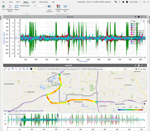
Figure 1. Using GPS map view to select the portion of the route to analyze.
After selecting the analysis range, we closed the map and added a displacement waveform. We also isolated the Strut(Z) channel by hiding the visibility of all other traces. The Traces pane is to the right of the main graph.
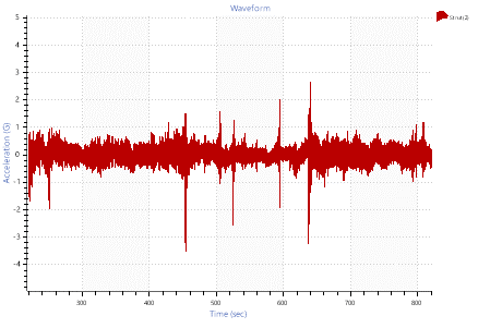
Figure 2. Acceleration data for the period of interest.
Both the acceleration and displacement traces had extended periods that fell primarily above or below zero. This trend indicated that there was low-frequency content in the waveform that would interfere with the displacement calculation (Figure 3).
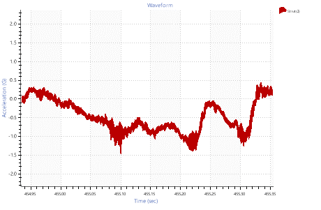
Figure 3. Low-frequency content that caused the acceleration data to stray from zero for extended periods.
In ObserVIEW, this low-frequency content can be removed from the acceleration waveform using a high-pass filter. We increased the filter corner frequency in increments until only the data of interest deviated the trace from zero (Figure 4).
To add a high-pass filter, navigate to the Trace Properties pane and select “Enable high pass filter.”
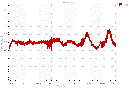
Figure 4. A high pass filter with a corner frequency of 10Hz removed low-frequency content.
After the acceleration data was filtered, we added a displacement graph. To add a new graph, navigate the Home tab and select Add Graph. Then, we slowly increased the corner frequency until the data appeared to be centered at zero.
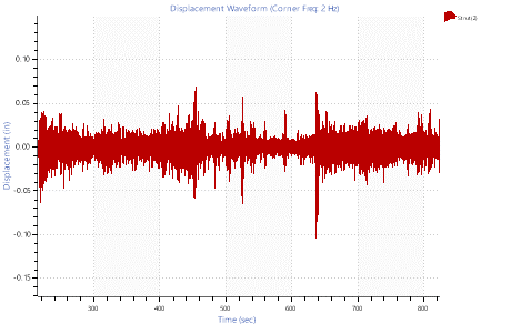
Figure 5. The acceleration data converted to displacement using a corner frequency of 2Hz.
Finally, the peak amplitudes in each direction were identified by placing a max and a min cursor near the peaks. To add a cursor to a graph, navigate to the Home tab and select Add Cursor.

Figure 6. Minimum and maximum values show displacement range.