Audio Playback
June 27, 2022
Back to: Getting to Know ObserVIEW 2022.1
Audio Playback plays back data audibly from the computer speakers or another PC device as an additional tool for analysis. It also works with a Live Analyzer connection. The sound of vibration data can help engineers validate a test profile or identify significant events.
Example 1
Using Audio Channels to Identify Events of Interest
Goal: To use the Audio Channels feature to listen to channels of interest and find sections of time data to analyze.
Software version: ObserVIEW 2022.1
Required licenses: Advanced
This analysis utilized a recording of a BMW driving on various roads/highways. The following adjustments were made to the analysis settings:
The graph traces were isolated to the rearview mirror traces, which were those of interest.
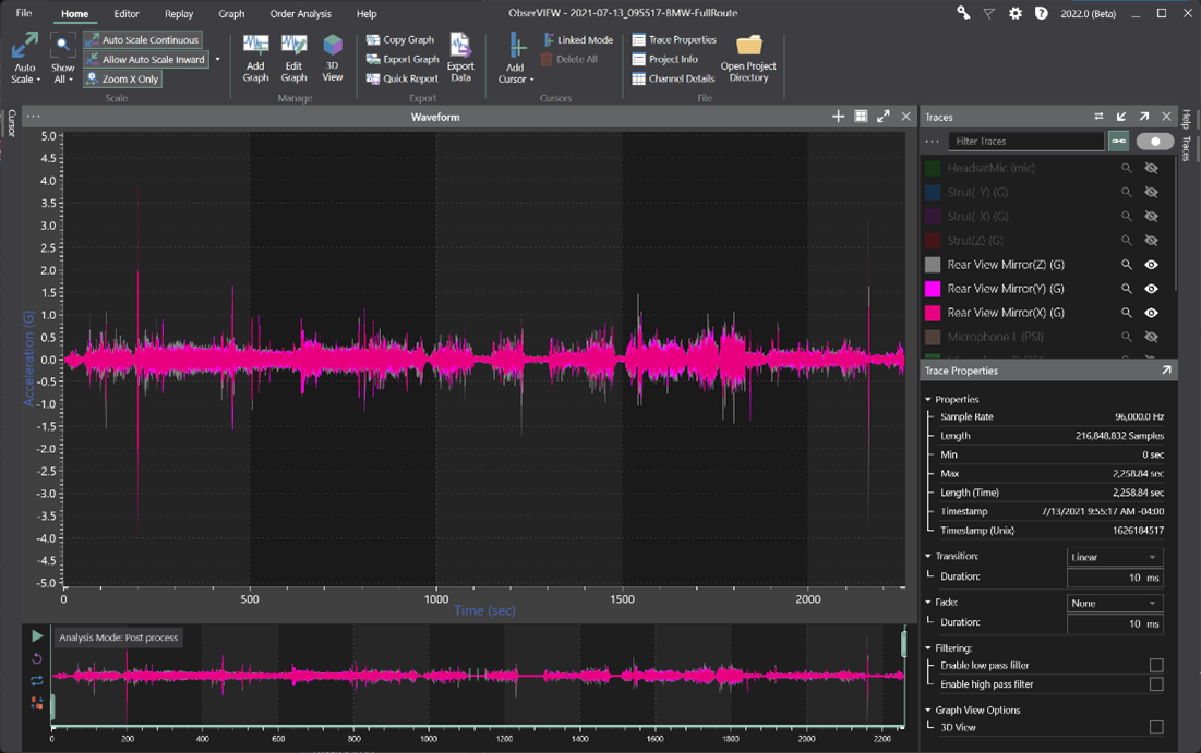
Isolated graph traces.
The MapVIEW tool was used to start the time range on highway M-6.
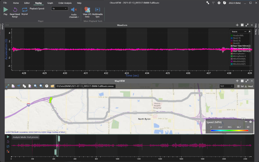
Adjusted time range.
The audio channels for the accelerometer attached to the rearview mirror were enabled.
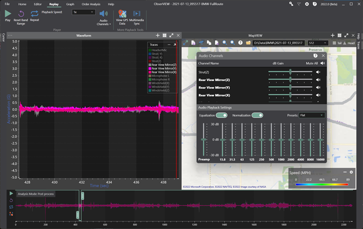
Enabled audio channels.
Then, we played the data back. There was irrelevant noise (i.e., road/wind noise), so the equalizer was used to filter out sound frequencies that were not of interest. We sought out noise from road bumps, so we filtered out everything above 1,000Hz and left everything below 1,000Hz at 0dB.
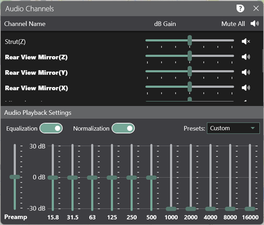
Audio Channels dialog.
We used headphones to listen for “bump” sounds in the data. We marked down the times to analyze later or paused and analyzed each instance as we heard them.
In one case, a bump noise occurred near 524.6 seconds, which matched an increase in acceleration that was visible on the waveform graph.
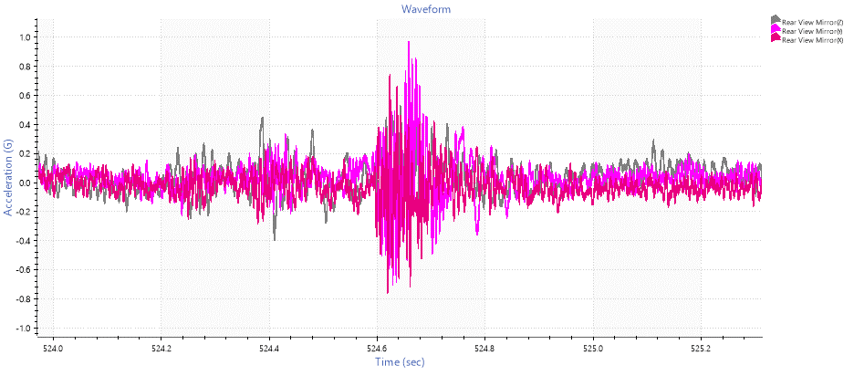
A “bump” noise near 524.6 seconds.
We used a theoretical specification to determine if the bump noise met the criteria. The specification stated that peak acceleration between 20 to 2,00Hz should be above 50Hz, and the displacement at that peak should be less than 0.005mm.
The fast Fourier transform (FFT) of the event was examined using the following settings:
- Min Frequency: 20Hz
- Max Frequency: 200Hz
- Analysis Lines: 16,384
- Window Function: Hanning
- Data Range Bias: Center
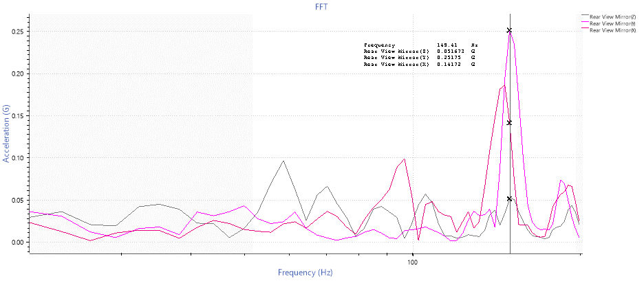
FFT of the event.
The peak acceleration was 149.41Hz, which meets the first part of the specification.
Next, a displacement FFT with a tolerance line at 0.005mm was used to determine if the displacement at that peak exceeded the specification. The max displacement at this peak was below 0.005mm, so the mirror met the specification for this event.
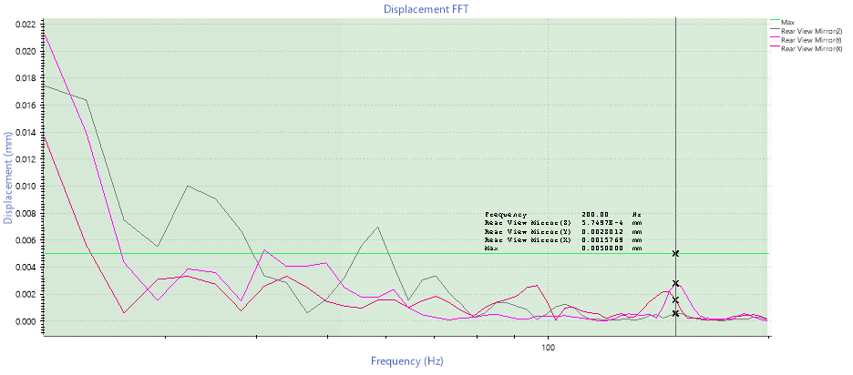
Displacement FFT with a tolerance line at 0.005mm.