Transfer Function Mathematics
March 19, 2019
Back to: Mathematics for Understanding Waveform Relationships
A transfer function, H(f), can be used to find resonance or anti-resonance in a system. Generally, the true transfer function is not known but can be estimated. A transfer function estimate is notated as Ĥ(f).
The transfer function indicates where there is a sudden increase (resonance) or decrease (anti-resonance) in the spectral power of a device or system.
A transfer function H(f) of a system with input (reference) x and output (response) y is written as the ratio H(f)=Y(f)/X(f), where X(f) is the Fourier transform of x and Y(f) is the Fourier transform of y.
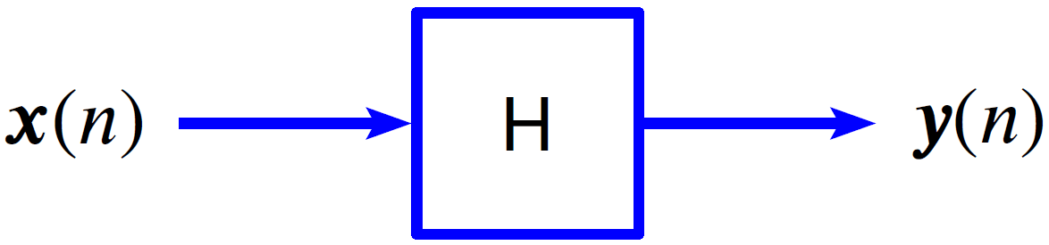
Figure 1.1. Graphical representation of a transfer function.
The transfer function H(f) tells us what is transferred from an input, X(f), to the output, Y(f). This is denoted as Y(f) = H(f)X(f).
If H is linear time-invariant (LTI), then a single frequency tone at the input will result in a single tone of the same frequency at the output, such that:
(1) 
and:
(2) 
In this case, it may well be that A1≠A2 and ϕ1≠ϕ2. Mathematically speaking, this means that sinusoids are eigenvectors of the linear operator H.
Estimating the Transfer Function
In general, the transfer function of a system is not known nor can be known. However, it can be estimated with a transfer function estimator Ĥ. There are several industry-standard estimators, including:
Ĥ1 “Least Squares Estimator”
Use Ĥ1 when the system has little or no input (reference) measurement noise.
Ĥ1 is especially applicable when driving (or forcing) the input with a shaker and a controller. The controller is in control of the input, so the input signal should be determined with very little measurement noise.
More details
When the input measurement noise is zero, Ĥ1 is the least-squares optimal estimate. In this case, selecting Ĥ1 is justified because it is a mathematically optimal ideal. In addition, when the system is LTI and the data is statistically stable (wide-sense stationary), the Ĥ1 is no longer just an estimate of H, it is precisely H (Ĥ1=H).
Ĥ2 “Inverse Method”
Use Ĥ2 when the system has significant input measurement noise but little or no output (response) measurement noise.
More details
When the output measurement noise is zero but the input noise is not zero, Ĥ2 is likely the optimal estimate. If there is no output measurement noise, H is LTI, and x is wide-sense stationary (WSS), then Ĥ2 is precisely H (Ĥ2= H).
In this scenario, however, Ĥ1 is biased relative to the true H. Ĥ1 = H/(1 + Suu/Sxx), where Suu is the power spectral density (PSD) of in the input noise and Sxx is the PSD of the measured signal. In this case, Ĥ1 is biased and underestimates H.
Similarly, if the input measurement noise is zero and output noise is greater than zero, Ĥ2 is biased relative to the true H. Ĥ2 = H(1 + Svv/Syy), where Svv is the PSD of in the output noise and Syy is the PSD of the measured output signal. In this case, Ĥ2 is biased and overestimates H.
If the input and output measurement noise are both zero, use Ĥ1, as Ĥ1 is the least-squares optimal estimate when the input noise is zero. When the input noise equals the output noise and both are zero, the system is LTI and the data is WSS. This means Ĥ1 = Ĥ2 = H and the ordinary coherence equals 1 (γ2(f) = 1).
Ĥv “Total Least Squares Estimator”
Use Ĥv if the noise power levels of the input and output are approximately equal but are not zero. If they are both zero, use Ĥ1 because Ĥ1 is the least-squares ideal estimator in this case.
Note that Ĥ1 ≤ Ĥv ≤ Ĥ2. Ĥv is somewhere between Ĥ1 (which tends to underestimate H) and Ĥ2 (which tends to overestimate H).
More details
Ĥ1 and Ĥ2 are extremes. Ĥ1 is ideal when input noise equals zero and Ĥ2 is ideal when output noise equals zero. Ĥv is somewhere in between.
(3) 
Txy “Transmissibility”
Use Txy to get a general idea of the ratio of output spectral-power to input spectral-power.
More details
Txy is the magnitude of the geometric mean of Ĥ1 and Ĥ2.
(4) 
Examples of Application
Ĥ1
Ĥ1 can be useful in seismic reflection near a peripheral noise source such as the ocean or a busy highway. Seismic reflection is used to map underground structures during searches for fossil fuels or aquifers. A shaker forces a signal into the ground with sensors located some distance away. The sensors receive seismic reflections of the shaker vibration as well as noise from the peripheral sources.
Ĥ2
Ĥ2 can be useful in situations where a low-sensitivity (i.e., high quantization noise, large input measurement noise) force transducer is mounted between a shaker and a massive device under test (DUT). A transducer is used for control and reference (input X). In addition, high-sensitivity (i.e., low quantization noise) accelerometers are mounted at critical response locations (outputs Y(n)) on the DUT. The result is an input/reference signal with large noise power and an output/response signal with no noise power. Ĥ2 is an ideal estimator in this case.
Ĥv
Similar to the Ĥ1 seismic reflection example, Ĥv can be useful in geophysical monitoring near a noise source such as the ocean or a busy highway. Geophysical monitoring predicts earthquakes and volcanic eruptions. The sensors receive signals from seismic activity and noise from peripheral sources.
Ĥv can also be useful in audio equalization (multiplication by 1/H) at a live concert. An audio engineer often needs to perform spectral equalization during a concert because the acoustics differ between an empty venue and a crowded one.
This involves calculating an estimate of the transfer function between two locations, such as the crowd mass center-left and center-right. The engineer uses two microphones, X and Y, suspended above the two locations, and then makes adjustments on the mixing board to introduce equalization approximately equal to 1/Ĥ. Measurements from both microphones will likely have significant, but approximately equal, power measurement noise due to ventilation equipment and the crowd. In this situation, Ĥv is a good estimator.
Txy
Txy can be useful during a comparison of the power of two signals, X and Y, emanating from two different devices and driven by two different shakers. In this case, the cross-spectral density should be zero or close to zero.
Example
- Begin with a shaker and beam test setup
- Put an input/reference accelerometer at the drive location and an output/response accelerometer at the end of the beam; the input measurement noise should be small, so select the Ĥ1 estimator
- Plot the magnitude of Ĥ1 as shown in Figure 1.2
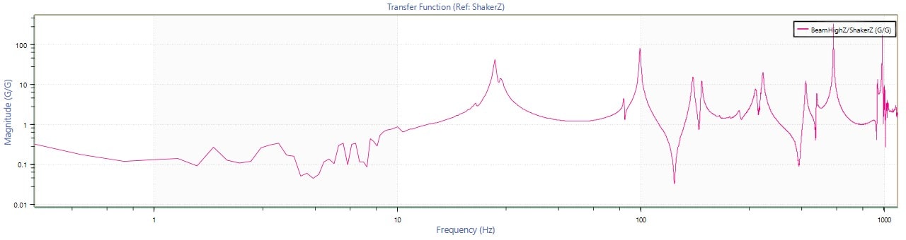
Figure 1.2: Transfer function graph.
- In Figure 1.2, there appears to be a resonant peak at 100 Hz. However, is it a resonance or just noise? To find out, generate a coherence function graph as shown in Figure 1.3
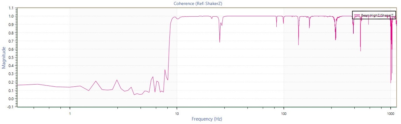
Figure 1.3: Coherence function graph.
- At 100Hz, the magnitude of the coherence is greater than 0.85. This indicates that the peak in Ĥ1 is due to resonance and not a spike in measurement noise
More Mathematical Details
It is not possible to know the true H(f) because, in general, systems are:
- not linear and/or
- changing over time (not time-invariant) and/or
- there is measurement noise (w and v in the diagram below)
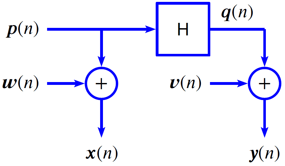
Figure 1.4: Transfer function with measurement noise inputs.
However, as previously discussed, it is possible to estimate H using one of several methods. Vibration Research’s ObserVIEW software package includes four H estimators. These estimators are, in turn, based on three other estimators. Specifically:
- Ŝxy(f) is an estimate of the cross-spectral density (CSD) of x and y
- Ŝxx(f) is an estimate of the power spectral density (PSD) of x
- Ŝyy(f) is an estimate of power spectral density (PSD) of y
Below are the exact definitions of the H estimators:
(5) 
(6) 
(7) ![\begin{equation*} H_{v}(f) = \frac{S_{yy}-S_{xx} + \sqrt{[\hat{S}_{yy}-S_{xx}]^2 + 4|S_{xy}|^2}}{2S_{xy}} \end{equation*}](https://vru.vibrationresearch.com/wp-content/ql-cache/quicklatex.com-83da0918a2176af58bfcba4313de7314_l3.png "Rendered by QuickLaTeX.com")
(8) 
Transfer Function Generalization
The transfer function estimators Ĥ1, Ĥ2, and Ĥv are all special cases of the more general scaled transfer function estimator Ĥs(f) with scaling factors, where 0 ≤ s ≤ ∞.