How to Compute the PSD
March 29, 2018
Back to: Random Testing
When computing the power spectral density (PSD) of a signal, it is essential to determine the frequency spectrum. Engineers can do so using the Fourier series, which is named after the mathematician Joseph Fourier who invented the method in 1807.
Fourier Series
The Fourier series is based on the principle that any signal x of length T can be constructed by the sum of a series of sine and cosine waves, each with an integer number of cycles in T. Mathematically, this is written as:
(1) ![\begin{equation*} x(t)=A_{0}+\sum_{n=1}^{\infty}[A_{n}\cos(2\pi f_{n}t)+B_{n}\sin(2\pi f_{n}t)] \end{equation*}](https://vru.vibrationresearch.com/wp-content/ql-cache/quicklatex.com-16597a22016699ad64ad191ba8e8b884_l3.png "Rendered by QuickLaTeX.com")
Equation 1
where f1 = 1 / T and fi = i f1. Ci and Si are the Fourier coefficients to be determined. Figure 2.6 illustrates this graphically.
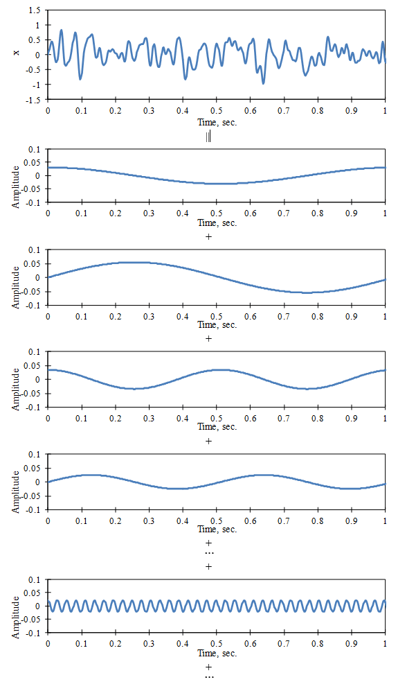
Figure 2.6. The Fourier series construction of a time signal.
In practice, the signal x is digitized into a sequence of N numbers (xn, n = 1 to N) with a time interval of Δt between samples (Figure 2.7).
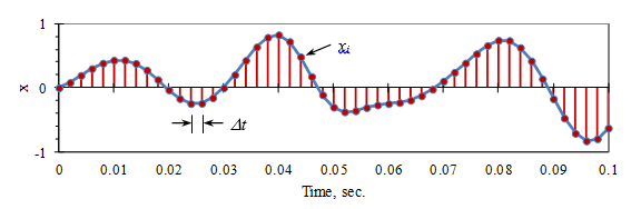
Figure 2.7. The digitization of a time signal.
Fourier Coefficients
We can determine the value of each Fourier coefficient by multiplying both sides of Eq. (1) by the corresponding sine or cosine wave and computing the mean value over N = T/Δt. Equation 2, for example, determines the value of C37.
(2) 
(3) ![\begin{equation*} =\frac{1}{N}\sum_{n=1}^{N}\cos(2\pi f_{37}t_{n})\left(\bar{x}+\sum_{i=1}^{\infty}[C_{i}\cos(2\pi f_{i}t_{n})+S_{i}\sin(2\pi f_{i}t_{n})]\right) \end{equation*}](https://vru.vibrationresearch.com/wp-content/ql-cache/quicklatex.com-d3ec69d02ae5e77836774f9f5962448c_l3.png "Rendered by QuickLaTeX.com")
Equation 2
The following summation computes the mean value and tn = n Δt:
(4) 
This procedure works because the different sine and cosine functions are independent of each other. That is, the mean value of the product of any two different functions is equal to zero, as illustrated in Figure 2.3. The terms in Equation 2 have a mean value of zero except for C37. Then:
(5) 
(6) 
(7) 
Equation 3
In Equation 3, the mean-square value of the cosine wave is 1/2 of what has been used (as illustrated in Figure 2.2). In general, the coefficients are determined by the following equation (Equation 4):
(8) 
(9) 
(10) 
Equation 4
Fast Fourier Transform
Historically, the computation of the summations in Equation 4 was very time-consuming until 1965, when Cooley and Tukey published an efficient algorithm for this known as the fast Fourier transform (FFT).
Their algorithm uses a sequence of N digital samples where N is a power of 2 (e.g. 2, 4, 8, 16, 32, etc.). The highest frequency that can be resolved in the FFT is fq = 1 / (2 Δt ) Hz (called the Nyquist frequency), so there are N / 2 frequency values. The signal x must be conditioned by a low pass filter before it is digitized to make sure that frequencies above fq have been removed.
The FFT computes the values of the Fourier coefficients Ci and Si. The mean square amplitude is given by ( Ci2 + Si2 ) / 2. Since the frequency resolution is Δf = 1 / T = 1 / ( N Δt ), the PSD is normalized to a 1Hz bandwidth by dividing the mean square amplitude by Δf.
(11) 
Equation 5
The process of generating a PSD must address a number of FFT computational details. These FFT details include digital time sampling, aliasing, windowing, frequency resolution, and averaging.