Module 2.3 – Kurtosion® vs. Traditional Random Test

Back to: VibrationVIEW Syllabus

Introduction

Modern vibration controllers assume a Gaussian distribution of data. Therefore, the peak accelerations produced in a test will be about three times the average acceleration values. In reality, however, actual peak accelerations found on the field can exceed three times the average accelerations.

Random tests using Gaussian distribution can under-test the device under test (DUT). In response, Vibration Research pioneered a novel technique to make tests more realistic. This patented technique of kurtosis control allows the test technician to adjust the kurtosis value (the value that dictates the probability of greater acceleration peaks to be present in the data) to a value that more realistically represents the peak accelerations found in the field.

Applying an appropriate kurtosis value to a test will make a test more realistic. Kurtosion^® can bring a product to failure more quickly without changing the test profile (See Sound and Vibration, October 2005, pg. 10-17). The following module runs a test at standard Gaussian distributions and compares the results to the same test run at a higher kurtosis value.

Procedure

Use the Hardware, Inputs, and System Limits configuration from Module 1.1.

1. Create an Advanced Random Test

a. Select New Test > Random.
b. Select Advanced.
c. Select Table and create a breakpoint table as displayed in the image below:

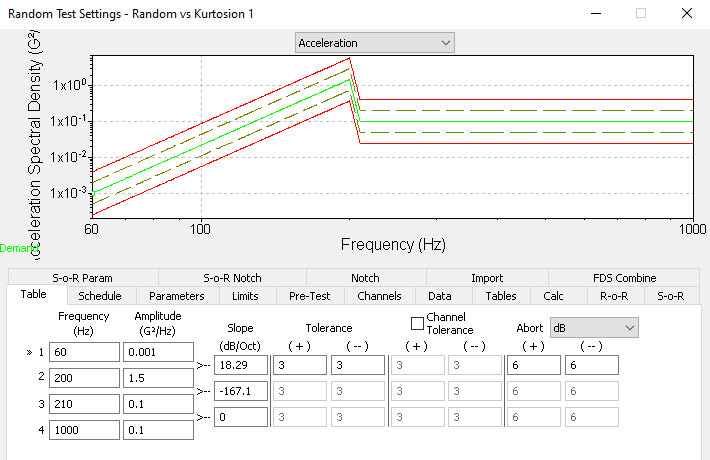
Frequency (Hz)
60
200
210
1000

Amplitude (G²/Hz)
0.001
1.5
0.1
0.1

d. Select Schedule and set the Run for time to 5 minutes.
e. Select Parameters, point to Sigma Clipping, and select No Clipping.
f. Select Limits and point to Running Drive Limits; set the Max system gain to 6 V/G and the Max output to 6 VRMS.
g. Select OK and save the test as Random vs Kurtosion 1.

2. Create the Graphs

a. Select New Graph
b. Graph 1 configuration

• Graph Type: Acceleration vs. Freq. (PSD)
• Graph Traces:
  • Control Loop Traces: Demand, Control, Tolerance, Abort
  • Input Channels: Ch1

c. Graph 2 configuration

• Graph Type: Acceleration Waveform
• Graph Traces:
  • Input Channels: Ch1

d. Graph 3 configuration

• Graph Type: Kurtosis
• Graph Traces:
  • Input Channels: Ch1

e. Graph 4 configuration

• Graph Type: Probability Density
• Graph Traces:
  • Input Channels: Ch1
  • Point to Axis Limits and change the y-axis to Log

f. Select OK.

3. Run the Test (1)

a. Listen carefully to the sounds produced by the test.
b. Watch the graphs, giving special attention to the PDF graph.
c. Save the data in an appropriate location.

4. Create a Report (1)

a. Select Report.
b. In the report, include the following information:

• Active Graph

c. Save the report as Random – NO KURTOSIS.
d. Select the Ch1 labels for the kurtosis waveform graph and the probability density function. Copy (Ctrl+c) the labels and then paste (Ctrl+v) them back onto the graph. This will create a permanent trace that will show the difference between each test.

5. Edit the Test (1)

a. Select Edit Test.
b. Select Parameters and change the following:

• Sigma Clipping
  • Method: Kurtosion®
  • Clip above: 20 Sigma
• Kurtosion
  • Kurtosis: 5
  • Transition Frequency: 100 Hz
  • Kurtosis Gain: 0.05

c. Run the test (2).
d. Select the Ch1 labels for the kurtosis waveform graph and the probability density function. Copy (Ctrl+c) the labels and then paste (Ctrl+v) them back onto the graph. This will create a permanent trace that will show the difference between each test.

6. Create a Report (2)

a. Select Report.
b. In the report, include the following information:

• Active Graph

c. Save the report as Random – K5.

7. Edit the Test (2)

a. Select Edit Test.
b. Select Parameters and change the following:

• Sigma Clipping
  • Method: Kurtosion®
  • Clip above: 20 Sigma
• Kurtosion
  • Kurtosis: 7
  • Transition Frequency: 100 Hz
  • Kurtosis Gain: 0.05

8. Run the Test (3)

a. Select the Ch1 labels for the kurtosis waveform and the probability density function. Copy (Ctrl+c) the labels and then paste (Ctrl+v) them back onto the graph.

9. Create a Report (3)

a. Select Report.
b. In the report, include the following information:

• Active Graph

c. Save the report as Random – K7.

10. Compare the Tests

Note the significant differences or similarities observed:

• In the PDF graphs, the tails of the kurtosis test are further from zero than the traditional test. This shows evidence that more of the higher peak accelerations are present in the kurtosis test.
• In the kurtosis waveform graphs: the kurtosis value for the traditional test is 3, which is typical of Gaussian distribution. The kurtosis value of the kurtosis test is 7, which matches the value set in the test parameters.
• In the acceleration waveforms, the peak accelerations are at approximately 3 G in the traditional test. The peak accelerations in the kurtosis test are greater than 5 G.

Questions to consider:

1. Are the PSDs the same for the traditional Gaussian test and the kurtosis control tests?

The acceleration profiles for both tests are identical because all other parameters are the same and the overall average power density is the same. Although the kurtosis test includes more of the higher accelerations peaks, the average power density remains the same because the smaller accelerations peaks have been lowered.

2.  Could you hear a difference between the traditional Gaussian test and the kurtosis control tests?

The traditional test emits a hissing sound. The kurtosis test has a similar hiss but with “popping” overtones. The reason for the popping is the higher acceleration peaks being introduced due to the kurtosis settings.