Module 2.4 – Kurtosion® with Varying Transition Band Frequency

Back to: VibrationVIEW Syllabus

Introduction

Increasing the kurtosis of a random vibration test improves the realistic nature of random testing. As noted earlier, many real-world vibrations are non-Gaussian and do not have peak accelerations greater than 3x the average vibration accelerations. Kurtosis control algorithms include many more peak accelerations in a vibration test. Therefore, it is necessary to match the kurtosis level of the test to the kurtosis level of the real-world vibration.

Kurtosis and the Transition Band Frequency

Many vibration control systems use different techniques to increase the kurtosis level of the random vibration test. However, the truly effective kurtosis techniques are those that adjust the transition band frequency.

The transition band dictates how long the random vibration test will dwell at higher amplitude vibrations. For example, a transition band value of 10,000 Hz introduces higher accelerations for only a very brief moment. These occasional, short-duration high accelerations are drowned out by the other vibrations in the test and, therefore, do not significantly increase the kurtosis of the test.

A lower transition band value, such as 5 Hz, introduces higher accelerations for a much longer period of time. These occasional, long-duration high accelerations are noticeably present in the test, and, therefore, increase the kurtosis of the test. Thus, to make a kurtosis control algorithm effective, it is necessary to adjust the transition band to a low value.

To what value should the transition band be set? There is a relationship between the bandwidth of the resonances and the transition band. The kurtosis control algorithm is most effective when the transition band is set to a value equal to the bandwidth of the resonances.

What effect will be observed with a decrease in the transition band? A test with a lower transition band dwells longer at the peak accelerations. Therefore, the device under test (DUT) will experience more of the large accelerations that are the cause of product failure. Lowering the transition band effectively increases the kurtosis value of the test, brings larger accelerations to the product, and, therefore, decreases the life of the product.

Procedure

Use the Hardware, Inputs, and System Limits configuration from Module 1.1.

1. Create an Advanced Random Test

a. Select New Test > Random.
b. Select Advanced.
c. Select Table and create a breakpoint table as displayed in the image below:

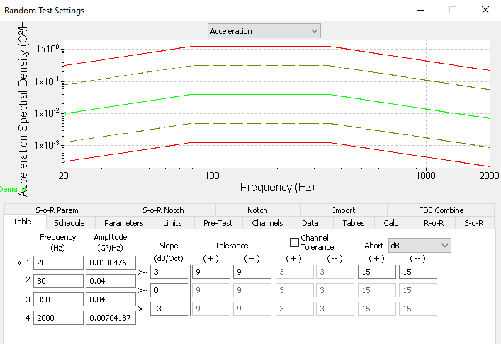
d. Set the tolerance limits to ± 9 and the abort limits to ± 15.
e. Select Schedule and set the Run for time to 30 minutes.
f. Select Parameters and set the following parameters:

• Sigma Clipping Method: Kurtosion®
• Clip above: 20
• Kurtosis: 70
• Transition Frequency: 1000 Hz
• Kurtosis Gain: 0.05

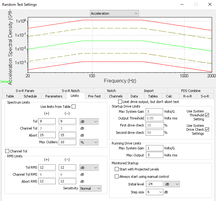
g. Select Limits and set the following limits:

• Spectrum Limits
  • Plus Abort (+): 15 dB
  • Minus Abort (-): 15 dB
  • Plus Tol (+): 9 dB
  • Minus Tol (-): 9 dB
• RMS Limits
  • Plus Abort (+): 12 dB
  • Minus Abort (-): 12 dB
  • Plus Tol (+): 12 dB
  • Minus Tol (-): 12 dB
• Startup Drive Limits
  • Max System Gain: 1 V/G
• Running Drive Limits
  • Max system gain = 1 V/G
  • Max output = 3 VRMS

h. Select OK and save the test as Name_KurtosionTB.

2. Create the Graphs

a. Select New Graph.
b. Graph 1 configuration

• Graph Type: Acceleration vs. Freq. (PSD)
• Graph Traces:
  • Control Loop Traces: Demand, Control, Tolerance, Abort
  • Input Channels: Ch1

c. Graph 2 configuration

• Graph Type: Acceleration Waveform
• Graph Traces:
  • Input Channels: Ch1

d. Graph 3 configuration

• Graph Type: Kurtosis
• Graph Traces:
  • Input Channels: Ch1

e. Graph 4 configuration

• Graph Type: Probability Density
• Graph Traces:
  • Input Channels: Ch1
  • Point to Axis Limits and change the y-axis to Log

f. Select OK.
g. Right-click on the kurtosis waveform graph, point to Annotate, and select Add Annotation. Double-click on the annotation and enter the following note: Kurtosis = [PARAM:CHkurtosis1]. Select OK.

3. Run the Test (1)

a. Allow the test to run for at least 10 minutes and listen carefully to the sounds produced by the test.
b. While the test is running, create a report with the following information:

• VibrationVIEW screen
• Demand, Control, Tolerance, Abort
• Breakpoint Table
• Current Measurements, Channel Measurements

c. When the test is finished, select the Ch1 labels for the kurtosis waveform graph and the probability density graph. Copy (Ctrl+c) the labels and then paste (Ctrl+v) them back onto the graph. Change the label to TB1000. This will create a permanent trace that will show the difference between each test.

4. Edit the Test (1)

a. Select Edit Test > Parameters.
b. Change the Transition Frequency to 100 Hz and select OK.

5. Run the Test (2)

a. Allow the test to run for at least 10 minutes.
b. While the test is running, create a report with the following information:

• VibrationVIEW screen
• Demand, Control, Tolerance, Abort
• Breakpoint Table
• Current Measurements, Channel Measurements

c. When the test is finished, select the Ch1 labels for the kurtosis waveform graph and the probability density function. Copy (Ctrl+c) the labels and then paste (Ctrl+v) them back onto the graph. Change the label to TB100.

6. Edit the Test (2)

a. Select Edit Test > Parameters.
b. Change the Transition Frequency to 10 Hz and select OK.

7. Run the Test (3)

a. Allow the test to run for at least 10 minutes.
b. While the test is running, create a report with the following information:

• VibrationVIEW screen
• Demand, Control, Tolerance, Abort
• Breakpoint Table
• Current Measurements, Channel Measurements

c. When the test is finished, select the Ch1 labels for the kurtosis waveform graph and the probability density function. Copy (Ctrl+c) the labels and then paste (Ctrl+v) them back onto the graph. Change the label to TB10.

8. Edit the Test (3)

a. Select Edit Test > Parameters.
b. Change the Transition Frequency to 2 Hz and select OK.
c. Change Sigma Clipping Method to No Clipping.

9. Run the Test (4)

a. Allow the test to run for at least 10 minutes.
b. While the test is running, create a report with the following information:

• VibrationVIEW screen
• Demand, Control, Tolerance, Abort
• Breakpoint Table
• Current Measurements, Channel Measurements

c. When the test is finished, select the Ch1 labels for the kurtosis waveform graph and the probability density function. Copy (Ctrl+c) the labels and then paste (Ctrl+v) them back onto the graph. Change the label to TB2.

10. Compare the Tests

a. The kurtosis waveform and PDF graphs have the most significant differences. As the tests are adjusted to a lower transition band frequency, they become progressively harsher on the product.

b. The acceleration profiles are identical for all data sets. The test settings are the same; therefore, the same amount of energy is being put into the tests.

It is important to note that the tests are identical in every regard except the kurtosis value. All tests are giving the same amount of energy to the product; therefore, the tests will not overwork the equipment in an attempt to break the product more quickly.

c. The PDF graphs all differ because of the changing of the transition band frequency. As the transition band frequency drops, the amount of acceleration on the product rises.

d. The kurtosis graphs are all roughly around 7. No clipping was set at 3 because it is the default Gaussian value. The tests with the lower transition band frequencies have a bit more variance in the kurtosis due in part to the higher accelerations present in these tests.

e. The acceleration waveform graphs are all different. A comparison of these graphs shows that higher acceleration vibrations are more prominent in the tests with decreasing transition band frequency.