Module 2.2 – Advanced Random Test

Back to: VibrationVIEW Syllabus

Use the Hardware, Inputs, and System Limits configuration from Module 1.1.

1. Create an Advanced Random Test

a.  Select New Test > Random.
b. Select Advanced.
c. Select Table and create a breakpoint table as displayed in the image below:

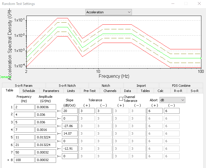
Frequency (Hz)
2
4
5
7
11
21
50
100

Amplitude (G²/Hz)
0.00036
0.036
0.036
0.0016
0.013224
0.013224
0.00032
0.00032

d. Select Schedule and set the Run for time to 7 m 30 s (7 minutes and 30 seconds).
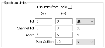
e. Select Limits.

• Point to Spectrum Limits and set the limits as displayed in the image below:

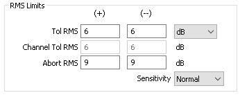
• Point to RMS Limits and set the limits as displayed in the image below:

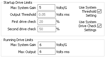
• Point to Startup Drive Limits and Running Drive Limits and set the limits as displayed in the image below:

f. Select OK and save the test as Name_AdvancedRandom.

2. Create the Graphs

a. Select New Graph.
b. Graph 1 configuration

• Graph Type: Acceleration vs. Freq. (acceleration spectral density)
• Graph Traces:
  • Control Loop Traces:
  • Input Channels: Ch1, Ch2
  • Select Show active lines

c. Graph 2 configuration

• Graph Type: Acceleration Waveform
• Graph Traces:
  • Input Channels: Ch1

d. Graph 3 configuration

• Graph Type: Probability Density
• Graph Traces:
  • Input Channels: Ch1
  • Point to Axis Limits and change the y-axis to Log

e. Select OK.

3. Run the Test

a. Autoscale the graphs as needed.
b. Listen to the test.
c. Save the data.
d. Compare the PDF graph to the Acceleration Waveform graph. The PDF graph corresponds well with the acceleration waveform graph. The majority of accelerations on the acceleration waveform graph are found at the ±0.5 G level. This is also seen in the probability density function. The majority of the area under the curve is found in the ±0.5 G region with minimal outliers.