Analyzing Random Vibration with the PSD
October 19, 2021
Fundamentals
Waveform Display
Domains for Analysis
Random Vibration
Back to: Introduction to Vibration Signals
A test engineer can proceed with vibration analysis after digitizing a continuous vibration signal into a sequence of numbers. As a random signal is not repetitive like sine, random vibration must be quantified with statistics or probability distributions.
Engineers typically analyze random vibration using the power spectral density (PSD). The PSD graph displays the distribution of a signal over a defined frequency spectrum. It reveals resonances and harmonics that are not readily available in a time-history graph.
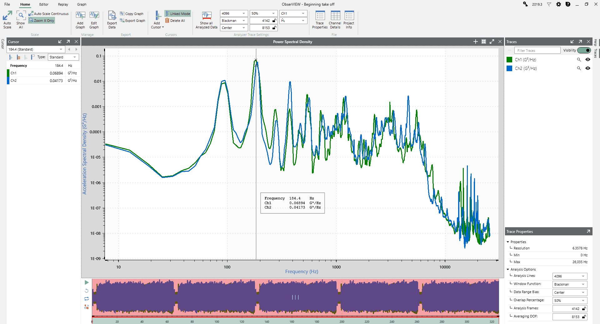
Power spectral density graph in ObserVIEW.
Magnitude of the PSD
The magnitude of the PSD is the mean-square value of the signal. It is normalized to a single hertz bandwidth, such as G2/Hz.
The mean value for any set of numbers is the sum of the numbers divided by the total amount of numbers in the set. It is often referred to as the arithmetic average. The mean square, then, is the mean squared value of a set of numbers.
The mean value of a signal’s amplitude is near zero. Thus, the values are squared to produce a positive quantity. To obtain a linear value, a square root is applied to the mean square. This calculation results in the root-mean-square (RMS) value.
Calculating the PSD
The frequency spectrum must be determined when computing the PSD of a signal, which can be achieved with the Fourier series.1 An algorithm known as the fast Fourier transform (FFT) is often used to compute the complex Fourier summations efficiently.2
To calculate the PSD from a time-history file, the algorithm partitions data into frames of equal length in time. The lines of resolution and sample rate can determine the frame width.
Next, the FFT transforms each frame to the frequency domain. The frequency-domain data are converted to power by computing the square magnitude of each frequency point. The squared magnitude for each frame is averaged. Then, the average is divided by the sample rate to normalize the magnitude to a single Hertz.
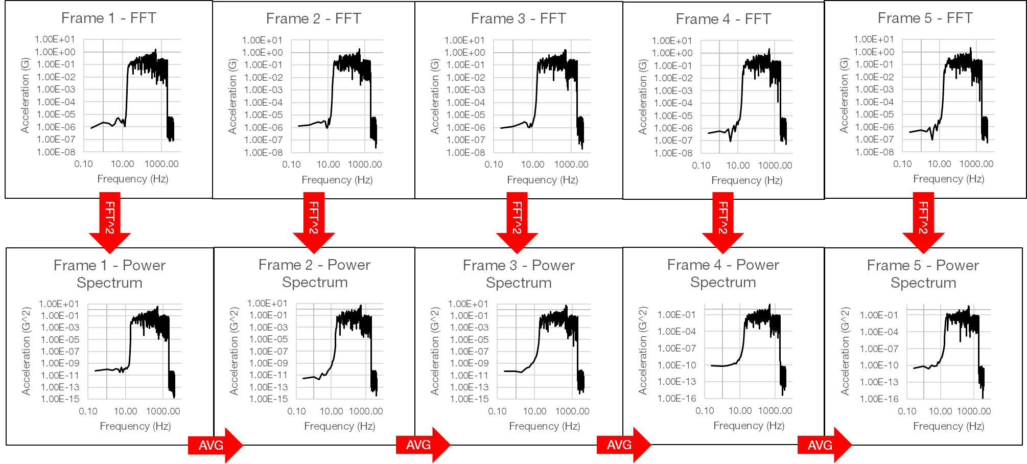
Overview of PSD calculation.
Welch’s Method
The Vibration Research software applies Welch’s method for PSD estimation, which uses the FFT algorithm to estimate the power spectra.3 An abridged description of the calculation is provided in this lesson. For a more in-depth discussion, take the lesson Calculating PSD from a Time History File.
Windowing
A window function is applied to the data before the FFT is employed. The FFT assumes data are an infinite series and considers the starting and ending points of each frame as consecutive. Random data are not often an infinite series, and a window function is necessary for such instances.
The frequency resolution of the PSD reflects the frequency spacing of the FFT: Δf = 1 / T, where T is the length of the time sample. A window function changes the frequency resolution and, therefore, the evaluation of resonance peaks.
The FFT of the windowed waveform is similar to the FFT of the original, but they are not equivalent. For a given frame width, the distortion characteristics of different window functions will vary.
Calculating the FFT on a Running Test
In statistics, degrees-of-freedom (DOF) is the number of values in the final calculation that are free to vary. When the PSD is calculated during a running test, there are two DOF for each framed FFT included in the PSD. The longer a test runs, the more framed FFTs are used to calculate the PSD. This increases the DOF that are characterizing the PSD.
When the PSD is calculated during a running test, the update interval is the time between successive FFT being included in the calculation. The update rate is the number of FFTs in the calculation per unit time.