Transfer Function
June 2, 2021
Process Data
Analyze Data
System Identification
Mathematical Foundations
Back to: Fundamentals of Signal Processing
A system is often characterized by a transfer function H(f). In general, H(f) is not known but can be estimated. A transfer function estimate, Ĥ(f), is an estimate of the true transfer function; that is, an estimate helps to identify a system and its properties.
A transfer function H(f) of a system with an input x and output y is a ratio where X(f) is the Fourier transform of x and Y(f) is the Fourier transform of y.
(1) 
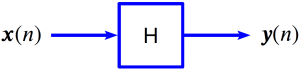
The transfer function helps to explain the transfer from the input X(f) to the output Y(f). That is, Y(f) = H(f)X(f).
If H is linear-time-invariant (LTI), then a single tone of frequency (f) at the input results in a single tone of the same frequency at the output.
(2) 
(3) 
(4) 
Mathematically, this means that sinusoids are eigenvectors of the linear operator H.
Mathematical Details
It is not possible to know the true H(f) because, in general, systems are not linear, change over time (not time-invariant), or have measurement noise.
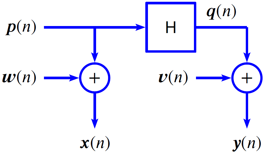
However, it is possible to estimate H. There are several ways to do so. Currently, ObserVIEW offers four estimators that are based on three other estimators.
- Ŝyx(f): estimate of the cross-spectral density (CSD) of y and x.
- Ŝxx(f): estimate of the power spectral density (PSD) of x.
- Ŝyy(f): estimate of the power spectral density (PSD) of y.
The following equations are the exact definitions of the transfer functions.
(5) 
(6) 
(7) ![\begin{equation*} \hat{H}_{v}(f)=\frac{\hat{S}_{yy}-\hat{S}_{xx}+\sqrt{[\hat{S}_{yy}-\hat{S}_{xx}]^2}+4|\hat{S}_{yx}|^2}{2\hat{S}_{yx}} \end{equation*}](https://vru.vibrationresearch.com/wp-content/ql-cache/quicklatex.com-b70cb47587b37d20103594e71bd830b6_l3.png "Rendered by QuickLaTeX.com")
(8) 
Features
Transfer Function Estimator Ĥ1
Ĥ1 is the least-squares optimal estimate when the input measurement noise is zero. In this case, using Ĥ1 is not just a rule of thumb but mathematically ideal.
When the system is also linear-time invariant (LTI), and the data is statistically stable (wide-sense stationary or WSS), then Ĥ1 is not just some estimate of the true H but is equal to H.
Transfer Function Estimator Ĥ2
Ĥ2 is likely to be the optimal estimate when the output measurement noise is zero, but the input is noise is not zero. If there is no output measurement noise, H is LTI, and x is WSS, then Ĥ2 is equal to H.
In the previous case, Ĥ1 is biased relative to the true H. Particularly, Ĥ1 = H/(1 + Suu/Sxx), where Suu is the PSD of in the input noise and Sxx is the PSD of the measured signal. That is, Ĥ1 is biased and under-estimates H.
Similarly, when the output measurement noise is zero, but the input is noise is not zero, Ĥ2 is biased relative to the true H. Particularly, Ĥ2 = H(1 + Svv/Syy), where Svv is the PSD of in the output noise and Syy is the PSD of the measured output signal. Ĥ2 is biased and overestimates H.
If the input and output measurement noises are both zero, the best selection is Ĥ1 because it is the least-squares optimal estimate when the input noise is zero. If input noise = output noise = 0, the system is LTI, and the data is WSS, then Ĥ1 = Ĥ2 = H. Moreover, the ordinary coherence γ2(f) = 1.
Transfer Function Estimator Ĥv
Again, if the input and output measurement noises are both zero, the best selection is Ĥ1. Note that Ĥ1 and Ĥ2 are extremes, as Ĥ1 is ideal when input noise = 0 and Ĥ2 for when output noise = 0. Ĥv falls somewhere in between Ĥ1 ≤ Ĥv ≤ Ĥ2.
As a generalization, Ĥ1, Ĥ2, and Ĥv are all special cases of the more general scaled transfer function estimator Ĥs(f) with scaling factor s, where 0 ≤ s ≤ ∞.
Transfer Function Estimator Tyx
Tyx is the magnitude of the geometric mean of Ĥ1 and Ĥ2.
(9) 