Filtering
June 2, 2021
Process Data
Analyze Data
System Identification
Mathematical Foundations
Back to: Fundamentals of Signal Processing
A filter is an operation that discriminates the components of an object over some domain. For example:
- In 3-dimensional space, filtering may include spatial discrimination: rejecting dirt and other large particles while admitting clean water to pass through.
- In the domain of time, Olympic qualifying races use temporal discrimination: rejecting slower runners while admitting faster ones.
Filtering
In statistics, filtering applies statistical discrimination. For example, a median-5 filter admits the median value of every set of five samples and rejects the other four. These filters are applicable to image processing and financial analysis.
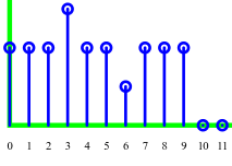
Input: 222322122200
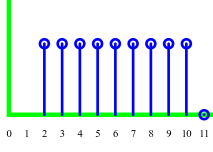
Output: 2222222220
In the frequency domain, filtering applies frequency discrimination. Filters reject or accept data components based on how frequently they change.
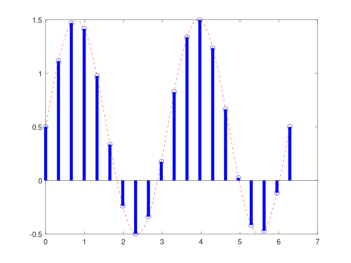
Input: Sinusoid + DC
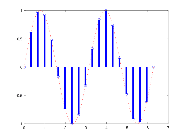
Output: Sinusoid only
Frequency Discriminating Filters
Apply a filter when you want to discriminate data based on frequency.
General Examples
- Rejecting (eliminate or filter out) frequency components.
- Accepting (admit or pass) frequency components.
- Boosting the energy level (magnitude) of some components.
Specific Examples
- Filtering out a DC offset (a constant offset)
- Filtering (notching) out 60Hz noise
- Filtering out components outside of a microphone, accelerometer, or other transducers’ specifications
- Filtering out components outside of an audio speaker or other shakers’ specifications
- Equalizing an audio recording by attenuating some frequency bands and boosting others
- Smoothing a noisy data sequence by attenuating rapidly changing (high-frequency) components
Types of Filter Operations
A filter performs some operation on a data sequence to yield a new sequence. The operation could be anything (or nothing in the case of an identity operation). However, there are some filters that engineers use so frequently that they have a title.
Low-Pass Filter
A low-pass filter attenuates high-frequency components above a specified corner frequency (fc) and allows low-frequency components below fc to pass through.
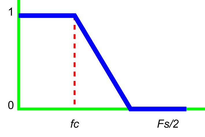
For example, a low-pass filter can clean up (or smooth) data contaminated with noise so that patterns are more readily apparent.
High-Pass Filter
A high-pass filter attenuates low-frequency components below a specified corner frequency and allows the high-frequency components above it to pass through.
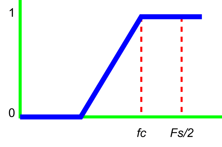
For example, if data have a large DC offset, a high-pass filter with a small corner frequency can remove the offset so that patterns of interest are more readily apparent.
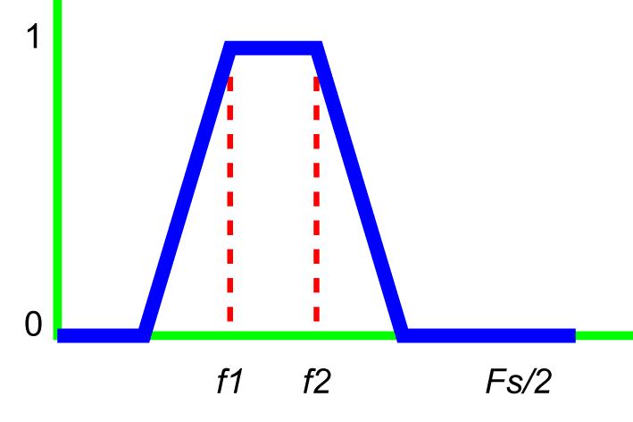
Bandpass Filter
A bandpass filter attenuates low and high frequencies and allows the middle frequencies to pass through.
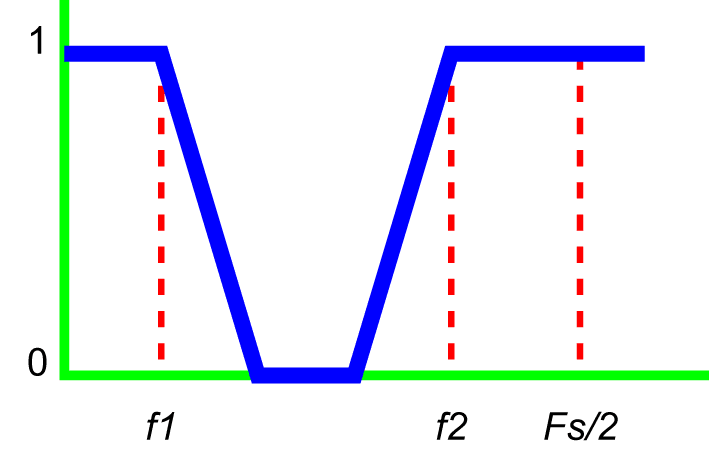
Notch Filter
A notch filter is the reverse of a bandpass filter. A notch filter rejects a band of frequencies and accepts everything outside the rejected band.
Filter Characteristics
Corner Frequency
Typically, the corner frequency of a filter response H(ω) is the frequency ωc, where the spectral power |H(ω)|2 has dropped from |H(ω)|2 = 1 to |H(ω)|2 = ½ or |H(ω)|=1/√2.
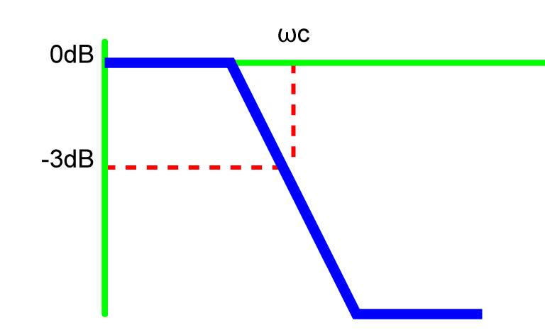
On a decibel (dB) scale, the spectral power drops from 10log10(1) = 0dB to:
(1) ![\begin{equation*} 10\log_{10}[|H(\omega c)|^2]=10\log_{10}(1/2) =-10\log_{10}(2) =-10\ln(2)/\ln(10) \approx-3.01\text{dB} \end{equation*}](https://vru.vibrationresearch.com/wp-content/ql-cache/quicklatex.com-4eb48ac1a9d6697938f1a95009d51ca0_l3.png "Rendered by QuickLaTeX.com")
Roll-Off
There are no perfect filters in the real world—that is, none drop straight down after reaching their corner frequency. Instead, they roll off at some slope. Real-world filters in the frequency domain are not like cliffs but like hills. This hill-like roll-off at the end leaves the upper 5% frequencies of the data invalid.
How Filters Work
Filtering in Time with Convolution
Often, a computer uses simple arithmetic to perform frequency-domain filtering. Specifically, each output y(n) is often a linear combination of inputs x(n). This type of filtering is called convolution.
For example, suppose we want to filter out direct current (DC). A simple filter with input x(n) and output y(n) will set y(n) = x(n) – x(n-1). Then, any DC signal at the input (x(n) = constant) will be filtered out because y(n) = constant – constant = 0.
Note: this filter is a digital differentiation.
Filtering in Frequency with Multiplication
Engineers may also filter a data sequence by first projecting it onto a basis. Often, this basis is a sequence of sines and cosines, and the tool for the projection is the fast Fourier transform (FFT).
According to the convolution theorem, filtering data in the time domain can be performed in the frequency domain by simple point-by-point multiplication. Before the multiplication in frequency can be carried out, we must first transform the data from time to frequency with the FFT.
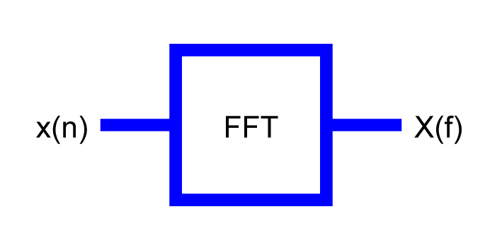
X(f) is the Fourier transform of x(n).
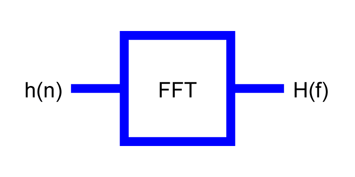
H(f) is the Fourier transform of h(n).
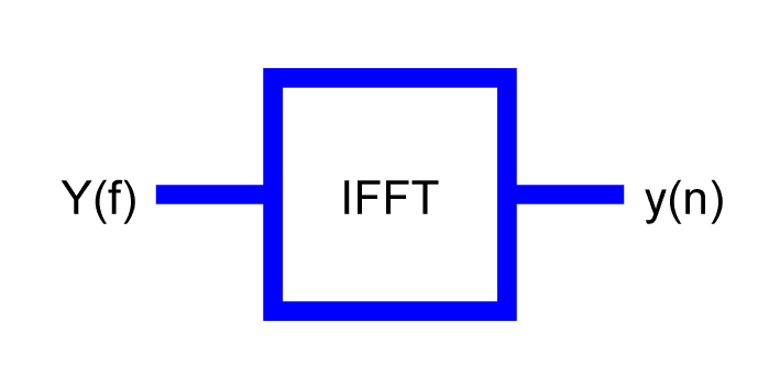
y(n) is the inverse Fourier transform of Y(f).
Filter Architectures
Mathematics and engineering often synthesize filtering using polynomials.
Mathematics: By the Weierstrass approximation theorem, any continuous function on a closed interval (0 ≤ time ≤ 10) can be approximated to arbitrary precision using polynomials.
Engineering: A polynomial can be implemented with addition and multiplication only. It is easy to implement both operations using digital logic gates in CPUs, DSPs, FPGAs, ASICs, etc.
For example, y = 5x2 + 3x + 2 means:
- Multiply 5 and x and x to get 5x2
- Multiply 3 and x to get 3x
- Add 5x2 and 3x and 2 to get y
Filters are often designed as polynomials over z, where z-n represents a delay by n samples. Therefore, the z-n factors can be implemented into hardware with a simple memory buffer.
Example
If a filter in the z-domain has the transfer function:
(2) 
(3) 
(4) 
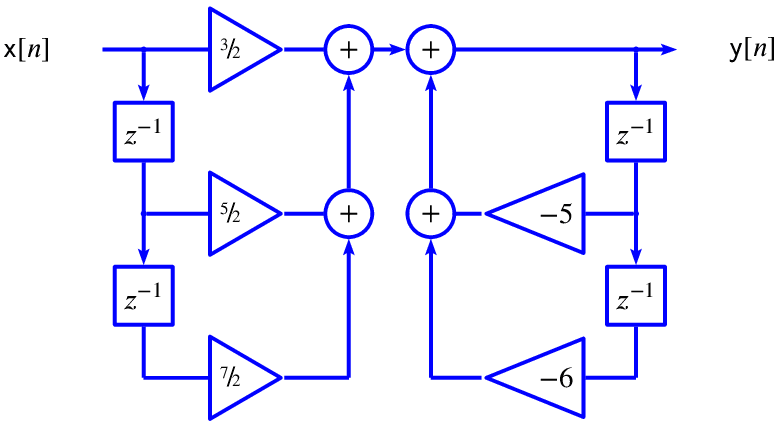
Then, in the z-domain:
(5) ![\begin{equation*} \text{Y(z)}[1+5\text{z}^{-1}+6\text{z}^{-2}]=\text{X(z)}\left[\frac{3}{2}+\frac{5}{2}\text{z}^{-1}+\frac{7}{2}\text{z}^{-2}\right] \end{equation*}](https://vru.vibrationresearch.com/wp-content/ql-cache/quicklatex.com-b0eafc89ed694c107b0d45033c3cbfb5_l3.png "Rendered by QuickLaTeX.com")
In the time domain:
(6) 
Therefore, at time n, the filter output y(n) equals:
(7) 