Coherence Mathematics
March 22, 2019
Transfer Function
Coherence
Cross Spectral Density
Back to: Mathematics for Understanding Waveform Relationships
Coherence indicates how closely a pair of signals (x and y) are statistically related. It is an indication of how closely x coheres or “sticks to” y.
In other words, coherence is how much influence events at x and events at y have on one another. The magnitude of coherence will always be between zero (no influence) and 1 (direct influence).
Mathematical literature defines two coherence functions.
Complex coherence:
(1) 
Ordinary coherence:
(2) 
where:
- Sxx(f) is the power spectral density (PSD) of x
- Syy(f) is the PSD of y, and
- Sxy(f) is the cross-spectral density (CSD) of x and y
Of the two definitions, ordinary coherence is more common in literature. However, ordinary coherence is the magnitude squared of complex coherence (γxy2(f)= |Cxy(f)|2). Thus, ordinary coherence is a special case of the more general complex coherence.
Applications of Coherence
In practical use, coherence has two main uses.
First, it establishes a measure of confidence that a peak observed in a transfer function is a resonant frequency of the device under test and not a spike due to measurement noise. For example, suppose that a peak at frequency f in a transfer function is observed. Then:
|
Ordinary Coherence |
|
Complex Coherence |
Description |
|
• γxy2(f) ≥ 0.70 |
or |
|Cxy| ≥ 0.85 |
A high degree of confidence that the peak is a resonant frequency. |
|
• γxy2(f) ≤ 0.50 |
or |
|Cxy| ≤ 0.707 |
Not likely that the peak is a resonant frequency. |
|
•0.50 < γxy2(f) < 0.70 |
or |
0.707 < |Cxy| < 0.85 |
Somewhat likely that the peak is a resonant frequency. |
Coherence also serves as a measure of a system’s linearity at frequency f. An ordinary coherence value close to 1 indicates that the system is linear time-invariant at frequency f. An ordinary coherence value close to zero indicates that the system is either non-linear, statistically changing with time, or both.
Note, if coherence drops within a resonance, the surrounding coherence values should be evaluated before making a judgment.
Example Walk-Through
- Start with a vibration test setup where the accelerometers can measure acceleration in the x and y directions across a range of frequencies. Generate the graphs shown as images in Figures 2.1, 2.2, and 2.3.
- To determine the spectral relationship between the x and y accelerations, use the transfer function estimators Ĥ1 and Ĥ2.
- Around 435Hz, both Ĥ1 and Ĥ2 exhibit remarkable gains. Initially, it may be assumed that 435Hz is a resonant frequency for Hxy.
- However, complex coherence equals 0.007, indicating that 435Hz is probably not a resonant peak.
- Conversely, the peak at 5330Hz does appear to indicate a resonant frequency, as there is a high coherence value in that vicinity.
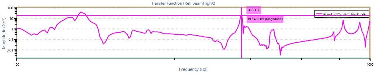
Figure 2.1. Ĥ1 transfer function graph.
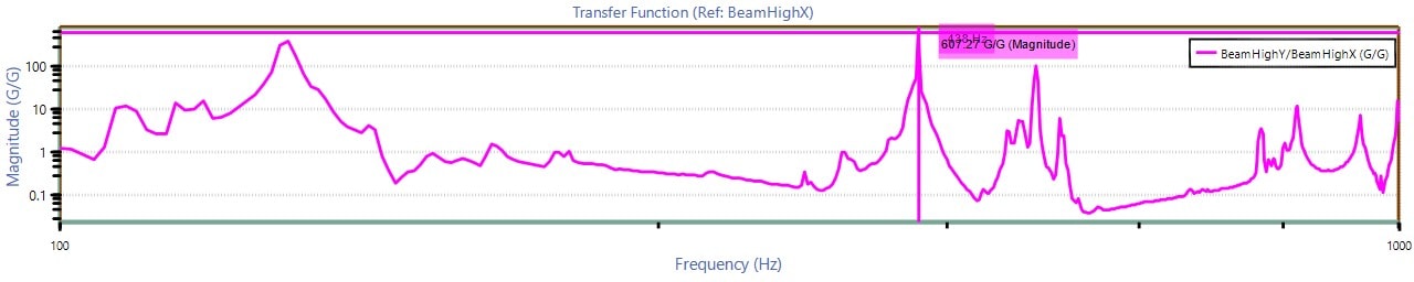
Figure 2.2. Ĥ2 transfer function graph.
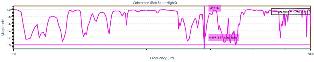
Figure 2.3. Cxy complex coherence graph.
Mathematical Details
Coherence as a Measure of Linearity
In many cases, the signal x may represent an input to a system (e.g., a device under test such as a mechanical device or the earth). The signal y may represent the output.
Suppose that an impulse to this system results in a response h[n] (the “impulse response”) and the discrete-time Fourier transform (DTFT) of this response is H(ω). If the system is linear time-invariant (LTI), then:
(3) 
The coherence will be:
(4) 
(5) 
(6) 
(7) 
(8) 
For a system that is linear time-invariant, the ordinary coherence γxy2(f) will be 1 for all frequencies. Conversely, if the coherence is less than 1, then it is not LTI. And, if γxy2(f) is 1 only at certain frequencies, then the system is LTI at those frequencies.
Coherence as a measure of confidence in transfer function H1
If a system is linear time-invariant with frequency response (Sxy(ω) = H(ω) Sxx(ω) ), then H(ω) = Sxy(ω)/Sxx(ω). This is the transfer function H1. To measure how “good” an estimator H1 is likely to be, check the ordinary coherence function γxy2(f). If γxy2(f) is 1 for all frequencies or close to it, then Hxy1(f) is likely a good Hxy1 estimator. If γxy2 is close to zero, then one should be much less confident about the quality of the Hxy1 estimator.
Coherence as a measure of distance between H1 and H2
The ordinary-coherence function γxy2(f) can also be viewed as a measure of the “distance” between Hxy1 and Hxy2. This is because:
(9) ![\begin{equation*} \gamma_{xy}^2=\frac{|S_{xy}|^2}{[S_{xx}S_{yy}]}=\frac{S_{xy}S_{xy}}{S_{xx}S_{yy}}=\frac{[\frac{S_{xy}(f)}{S_{xx}}]}{[\frac{S_{yy}}{S_{xy}}]}=\frac{H_{1}}{H_{2}} \end{equation*}](https://vru.vibrationresearch.com/wp-content/ql-cache/quicklatex.com-e1ce6783b66d7b4097ef39cb18fe24f2_l3.png "Rendered by QuickLaTeX.com")
(10) 
By using the ordinary-coherence function, the distance between |H1(435)|=19 and |H2(435)|=607 is very great. This is reflected in the following equation:
(11) 