Analyzing Random Vibration Data
July 22, 2024
Initial Design
Data Analysis
Reporting
Back to: Making Sense of Test Data
Many applications fall under the umbrella of random vibration data analysis. The analysis type an engineer selects largely depends on the device under test, end-use environment, and test goals. However, some considerations can be applied universally. This lesson offers general starting points for analyzing random vibration data.
Importing data into an analysis program can occur in several ways. A vibration control software program may provide sufficient displays and analysis tools for vibration test data, or the engineer may need to export the data to analyze in a separate program. For example, the ObserVIEW analysis software supports .txt, .csv, .uff, .wav, .vfw, and .mat files.
Graphs
Vibration analysis software programs include many graph types for reviewing data, the default typically being a time waveform. Each graph trace represents a test output as well as the control and demand signals.
Time Domain, Frequency Domain, and Waterfall Graphs
Engineers typically analyze vibration data in the time and frequency domains.
A signal in the time domain displays a measured parameter (acceleration, velocity, displacement, etc.) as a function of time. Engineers can use this data to identify data anomalies, test setup issues (such as cable disconnection), or visualize time-varying behavior, such as amplitude changes due to resonance or damping.
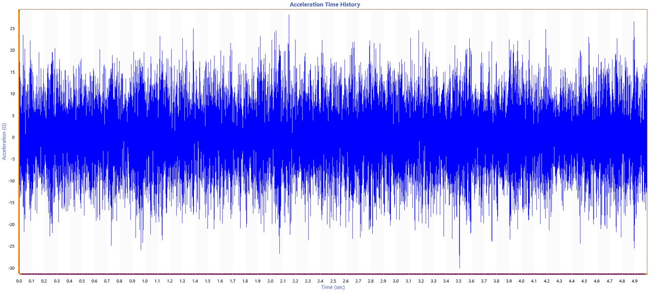
Random acceleration time history graph.
For a more in-depth analysis, engineers transform the data to the frequency domain.
Frequency Domain Graphs
Information obscured in a time-history waveform is often visible in the frequency domain. As most systems measure vibration signals in the time domain, time-domain data must be transformed for frequency-domain analysis. A standard algorithm can move the time-domain data to a different domain. One of the most popular is the fast Fourier transform (FFT).
In the frequency domain, engineers can observe the frequency content of the time-history waveform and gather information such as excitation frequencies, peak acceleration and distribution, and harmonic content.
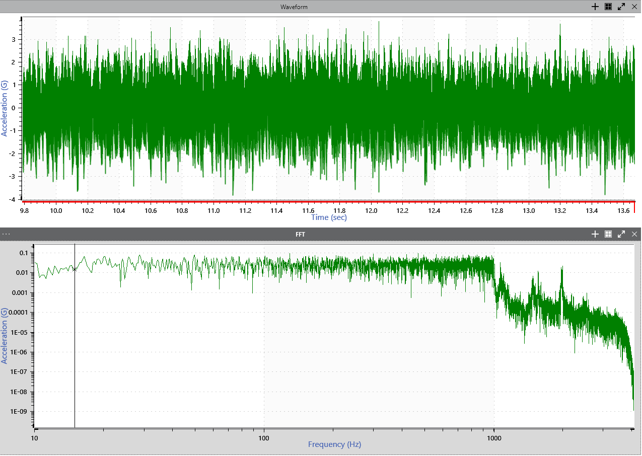
Random acceleration time waveform and FFT.
When applying an algorithm such as the FFT to time-history data, parameters such as the sample rate and windowing affect the resulting content. The Settings for Analyzing Vibration Signals lesson walks through the general parameters of analyzing random vibration signals, particularly when converting time data to the frequency domain.
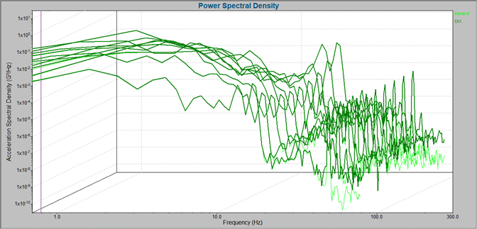
Power Spectral Density
The power spectral density (PSD) is an industry-standard frequency-domain graph for analyzing random vibration. It estimates the distribution of signal strength across a frequency spectrum and is a powerful tool for characterizing random vibration.
A frequency-domain graph such as the PSD allows engineers to determine which frequencies contribute most to the overall vibration energy, helping to identify dominant frequency components and potential resonances. With this information, engineers can assess performance under real-world conditions and design appropriate damping or isolation measures.
The Calculating PSD from a Time-history File lesson summarizes the process of the PSD calculation, including relevant parameters.
Other Frequency-domain Graphs
Many other graphs are available in the frequency domain, including:
- Transmissibility: amplitude ratio between an output and input across a frequency range
- Transfer function: estimated output from a given input; indicates phase differences between signals
- Coherence: statistical relationship between two signals at a set frequency value based on phase differences
The VibrationVIEW Analyzer Software Package course reviews the function of these advanced graph options.
Waterfall Graph
To review the change in frequency over time, an engineer can plot data as a waterfall graph. A waterfall plot is a series of spectral maps captured at regular time intervals.
Waterfall plots show the change in frequency over time and the scale of change in acceleration, velocity, or displacement, etc. It can provide more information about the overall test than an individual trace.
A time-frequency waterfall graph may be beneficial when:
- Measuring the changes in vibration as a machine load changes
- Identifying resonant behavior over time or a fundamental bending mode frequency
- Seeking to maintain constant conditions
- Monitoring shifts in resonant frequency
- Looking for orders on rotating machinery
Statistics
A visual overview of a time or frequency graph only offers so much information. Engineers calculate statistics for a comprehensive look into a device under test’s (DUT) behavior. The following are several notable statistics in random vibration data analysis.
Root-mean-square
The PSD is a statistical estimation of a signal’s distribution of power over a defined spectrum. The root-mean-square (RMS) of a PSD measures the spectrum’s overall random vibration acceleration. Generally, it is an accepted metric for average test intensity.
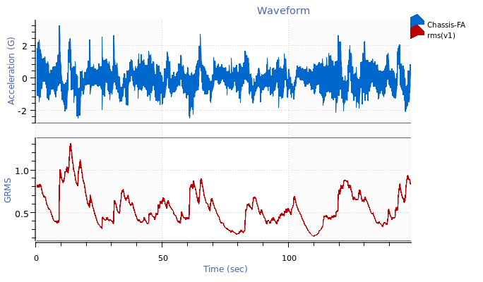
Acceleration waveform and RMS math trace.
After a PSD is generated with a fixed frequency resolution, its RMS value remains constant. This consistency allows engineers to match a PSD to a specification and determine if the RMS meets requirements. They can also use the RMS to compare two PSD plots with the same parameters and verify that they measure the same amount of energy.
Engineers can calculate the RMS (a single numerical value) from data recorded during a random vibration test. Then, they can compare the test RMS to the DUT’s acceptance criteria. For example, the criteria may specify the maximum allowable RMS levels for different operating conditions. If the RMS values exceed the specified limits, further investigation may be required to identify potential design flaws.
Peak Level
Peak level is the signal’s maximum amplitude. Engineers identify peak values to assess potentially damaging levels and compare them to specification boundaries. For example, some specificants require engineers to define the top 10 peak values.
While RMS is a convenient measurement of the overall strength of a signal, it is a mean value. Peak values, on the other hand, can inflict the most significant damage on a DUT, so engineers may review them without the averaging effect in the RMS value.
Crest Factor
Practical testing only considers random motion bound by a crest factor, which is expressed as a ratio between the absolute maximum of the signal and the RMS. The crest factor can be determined based on the test’s desired kurtosis value. It offers insights into signal shape and the potential for transient events.
Kurtosis
Kurtosis describes the deviation of a data set’s peak values from a Gaussian distribution. Random vibration with a normal distribution has a kurtosis of 3. Values greater than 3 indicate high-energy peaks over 3 sigma (standard deviations) from the mean value and may point to more damaging behavior.
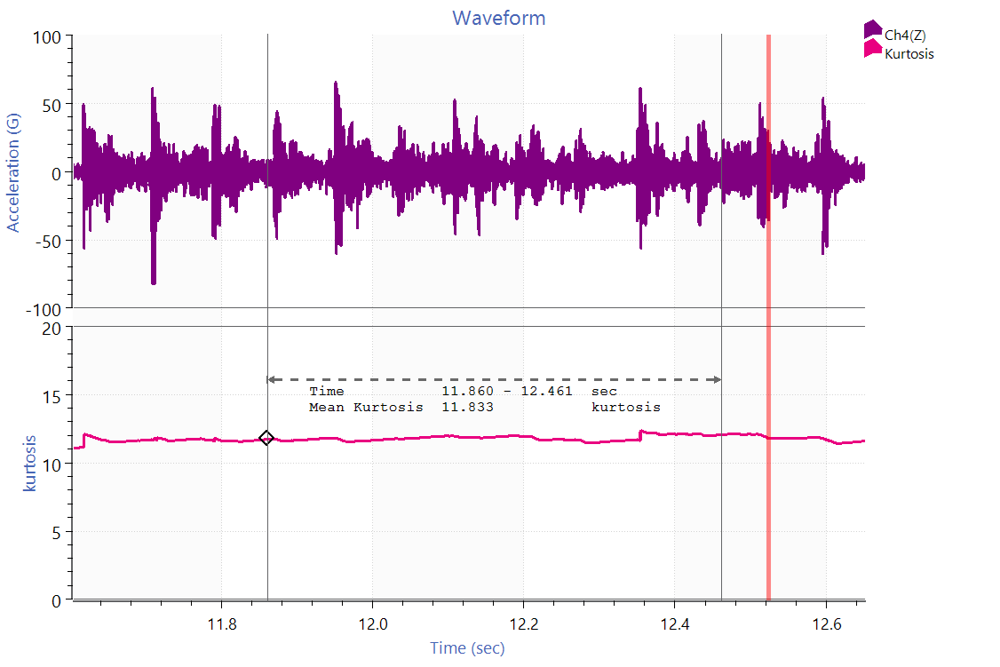
Acceleration time waveform and mean kurtosis math trace.
Engineers can calculate kurtosis (a single numerical value) from acceleration data recorded during a random vibration test. If the value is higher than anticipated, the signal may have more extreme outliers than a normal distribution would predict.
The engineer may investigate further to determine the cause of the high kurtosis. They might examine the vibration waveform for any irregularities, inspect the test setup for sources of non-linearity or resonance, or compare the results to previous tests.
Kurtosis offers valuable insights into the behavior of the DUT and helps identify potential issues or areas for improvement.