Transfer Function Graph
January 2, 2019
Getting Started with Analyzer
Primary Graphing Functions
Back to: VibrationVIEW Analyzer Software Package
Transfer function is an Analyzer graph option in the VibrationVIEW Random and Shock test modules.
The transfer function represents a linear, time-invariant system, where the input signal generates a homogeneous output. It defines the output that the system should produce from a given input.
 The transfer function is an estimate because, in general, systems are not linear, change over time, or include measurement noise. This estimate describes an ideal scenario where the test shaker perfectly transmits the drive signal to the test item, and the test item responds as anticipated. A significant deviation from the transfer function estimate can indicate an issue with the system’s stability or the presence of signal disturbances.
A graph of the transfer function displays the ratio of cross-spectra values for two signals in a defined frequency range. It also shows the phase relationship between the signals. In the VibrationVIEW software, the user can compare two input channels or one channel and the drive (output) signal.
Transfer Function Graph
VibrationVIEW computes the transfer function plot using the average cross-spectra for a series of waveforms (Random) or pulses (Shock). A ratio value of 1 indicates that the signals have the same acceleration. Values other than 1 indicate a difference in acceleration at that frequency.
The transfer function plot delivers valuable insights for vibration testing. During setup, it can help the engineer determine if the shaker head’s vibrations meet the reference values and troubleshoot for test/system anomalies.
 For example, imagine two accelerometers on a shaker head: one at the center and one at the edge. The test engineer can compare the response signals from the accelerometers and determine if the shaker head is moving consistently up and down without tilting, rotating, or flexing.
After running a test, they can use the graph to identify resonances and determine acceleration and phase relationships between signals. If the response deviates from what was anticipated, the engineer can look for disturbances such as noise.
Phase Value
The transfer function graph also indicates phase differences between signals. If it has a phase value of 0o, the accelerometers are moving in phase. A value of 180o indicates that they are moving 180o out of phase. Any other value signifies that they are in another off-beat phase.
Transfer Function vs Transmissibility
A transmissibility graph also displays the cross-spectral relationship between two signals. However, the phase relationship is unique to the transfer function option. The transfer function also uses more complex algorithms that result in smoother data. For more information on transfer function estimates, visit the Transfer Function Mathematics lesson.
To compare the transfer function graph with the transmissibility graph, consider the following:
An engineer runs a test to compare the acceleration of a shaker head and the device under test (DUT). The transfer function graph has a ratio value of 1 across the spectrum. The transmissibility graph also has a value of 1.
Given the ratio value, the engineer may conclude that the shaker head and the DUT are vibrating at the same acceleration.
With a plot of the transfer function phase, however, the engineer can determine if the shaker head and DUT are moving in the same direction at the same time. The transfer function can have an acceleration ratio value of 1 and a phase value of 180o, which would indicate opposite directions of motion with the same acceleration.
Example
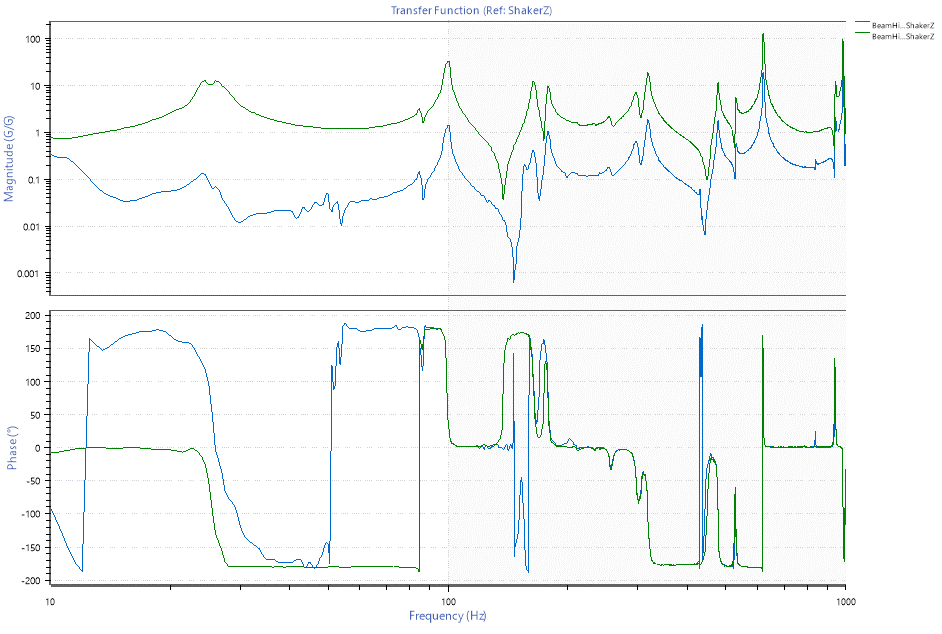
In Figure 2.1, the phase ratio of the two channels is 0o for the first 80Hz, indicating that the two accelerometers are moving in the same direction. As the aluminum beam approaches a major resonance, the phase ratio rapidly changes. At peak resonance, the phase ratio is 90o. For the remainder of the test, the phase ratio oscillates between 180o and -180o. These values indicate that the aluminum beam and the shaker head vibrated in the same direction for only a short period.
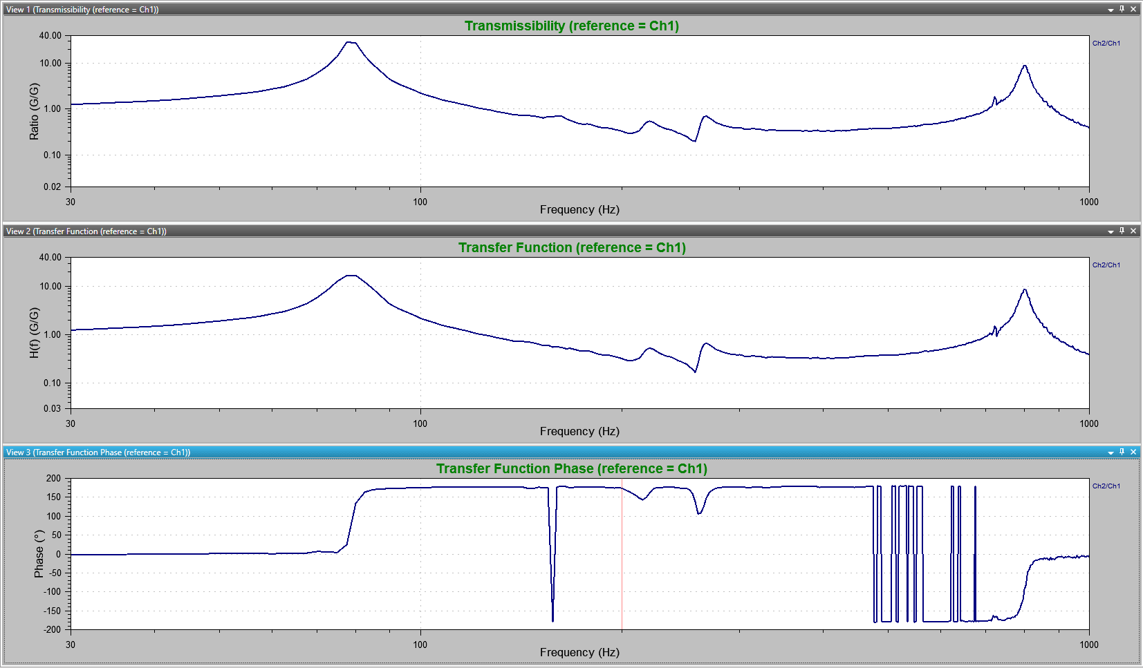
Figure 2.1. Transmissibility (above) compared to the transfer function (below) for beam vibrations (Ch.2) and shaker head vibrations (Ch. 1). For a majority of the frequency spectrum, the aluminum beam is vibrating out of phase (180o or –180o) with the shaker head.
Graph Comparison
The following test results are from a vibration shaker test. Channel 1 is the control acceleration, and Channel 2 is the response of a cantilever beam. The resulting transfer function and transmissibility graphs display the acceleration ratios of the two accelerometers (Figures 2.2 and 2.3).
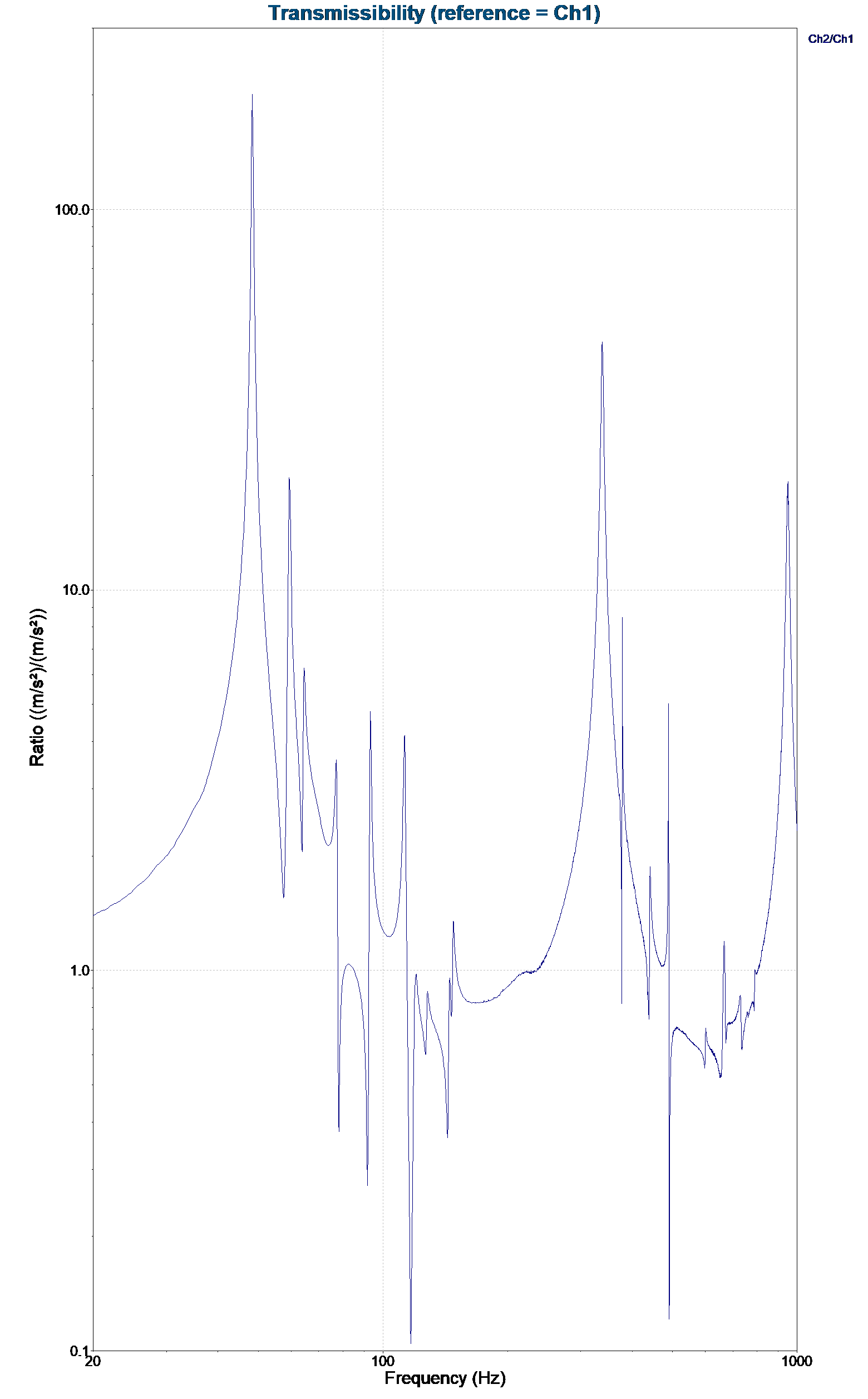
Figure 2.2. Transmissibility plot of control acceleration (Ch1) and the response of a cantilever beam (Ch2).
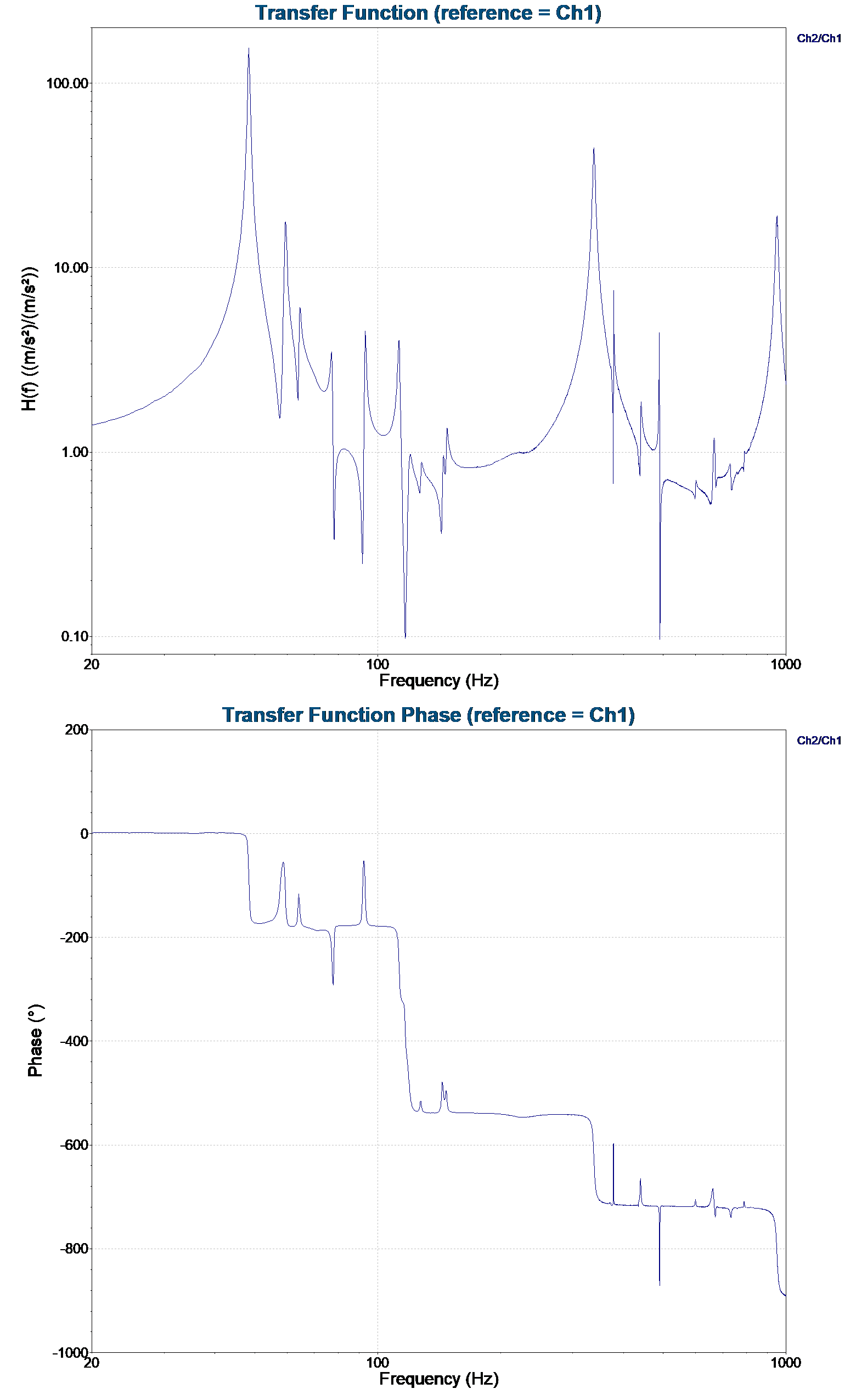
Figure 2.3. Transfer function plot and phase of control acceleration (Ch1) and the response of a cantilever beam (Ch2).
This transfer function (amplitude) graph is essentially identical to a transmissibility plot because they both compare the acceleration ratios of the two accelerometers. However, the transfer function phase provides more information regarding phase relationships.
The transfer function graph has two advantages over one for transmissibility. First, a plot of the transfer function phase provides information about the phase relationship between the signals. Second, the transfer function acceleration ratio is more accurate than the transmissibility graph because it effectively removes the noise factor.
The major disadvantage of the transfer function is the computation time needed. They are more complex than the calculations for the transmissibility graph.