Q-Factor

March 29, 2018

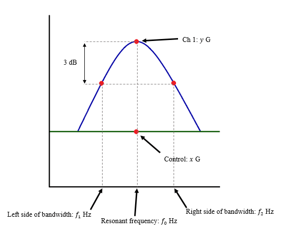
The Q-factor of a resonance is the ratio of the resonance’s center frequency to its half-power bandwidth. It tells us how sharp, or steep, the resonance is.

(1) $\begin{equation*} \text{Transmissibility}=\frac{\text{Ch}1}{\text{Control}}=\frac{yG}{xG} \end{equation*}$

(2) $\begin{equation*} \text{Q-factor}=\frac{\text{Resonant frequency}}{3dB \text{ bandwidth}}=\frac{f_{0}\text{Hz}}{f_{2}-f_{1}\text{Hz}} \end{equation*}$

Example

For example, if the center frequency of a resonance value was 97.91Hz, the equation to solve the Q-factor would be:

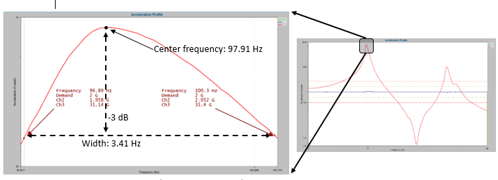
(3) $\begin{equation*} Q=\frac{\text{resonance center frequency }(f_c)}{-3dB\text{ bandwidth }(BW)}=\frac{97.91Hz}{100.3Hz-96.89Hz}=\frac{97.91Hz}{3.41Hz}\approx 28.7 \end{equation*}$

calculation for the Q-factor of a resonant frequency

Figure 4.2. Q-factor of a resonance (with some approximation).

Resonance Sharpness

In Figure 4.3, the left graph displays resonances with the same amplitude and center frequency but varying bandwidths. Notice the difference in sharpness between the three curves.

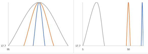
graphical representation of the Q-factor for different resonant frequencies

Figure 4.3. Q-factor for several resonances. On the left are identical frequencies with varying bandwidths. On the right are identical bandwidths with varying center frequencies (logarithmic axes).

The right graph displays resonances with the same amplitude and bandwidth but varying center frequencies. On a linear axis, the difference in sharpness is not evident. However, it is on a logarithmic axis.

Example

Let’s refer back to Figure 4.1. The Q-factor was:

25.4 for the 67.99Hz resonance
12.4 for the 142.1Hz resonance
68.5 for the 538.1Hz resonance

The 538.1Hz resonance was the sharpest.

The sharper the resonance, the quicker the resonance will resonate during a sine sweep and the harder it is to control. The Q-factor measures the difference between a resonance that slowly ramps up during a sine sweep (a wide resonance with a low Q-factor) and a resonance that quickly ramps up (a sharp resonance with a high Q-factor).

The excitation frequency does not need to equal a resonant frequency to cause amplification. Even nearby frequencies (±10%) can agitate some amplification. Therefore, resonances can increase in amplitude before and after the resonance peak. A resonance peak can be sharp or broad, depending on the structure’s damping.

Additional Measurements

In addition to FFT-related plots, other information, such as transmissibility and phase, confirms resonances and defines the most damaging frequencies.

Transmissibility

A transmissibility graph displays the amplitude ratio between two channels—i.e., input vibration to output response as a function of frequency. When searching for resonances, the transmissibility plot indicates which frequencies generate an amplified response, indicating a resonance. A DUT’s maximum transmissibility occurs at its natural frequency with no damping.

Phase

At resonance, the excitation and response are, theoretically, 90 or 270 (-90) degrees out of phase. Realistically, the phase difference will typically be near to, but not exactly, ±90 degrees because of material imperfections, accelerometer mounting locations, and non-linear shaker motion. The phase difference may also shift due to changes in test amplitude or non-linear responses to fatigue.