DSP Calculus
June 2, 2021
Process Data
Analyze Data
System Identification
Mathematical Foundations
Back to: Fundamentals of Signal Processing
In many cases, the physical world is ruled by differential relationships. For example:
- Velocity = d/dt displacement
- Acceleration = d/dt velocity
- Current through a capacitor = capacitance (C) times d/dt of the voltage across the capacitor
Digital Differentiation
Differentiation (d/dt) is built for the analog world or continuous functions, not for the digital signal processor (DSP) one (discrete functions or sequences). By definition:
(1) 
If x(t) is continuous, then x(t) and x(t-h) can get closer while h gets closer to 0. However, if x(n) is discrete, then the smallest h can be is 1, and the closest the numerator can get is x(n)-x(n-1).
That is, the resolution of digital differentiation is limited by the sample rate Fs.
How accurate is discrete differentiation compared to continuous differentiation? It is helpful to compare them in the frequency domain.
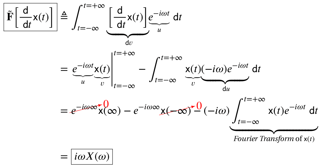
The Fourier transform of d/dt is iω because:
The z-transform of y(n)=x(n)-x(n-1) is Y(z) = X(z) – z-1X(z). Therefore:
(2) 
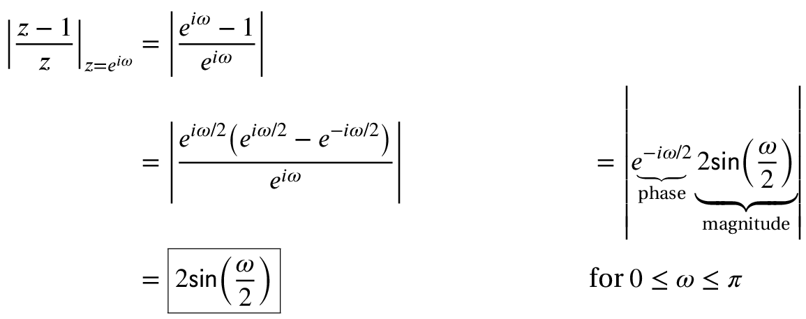
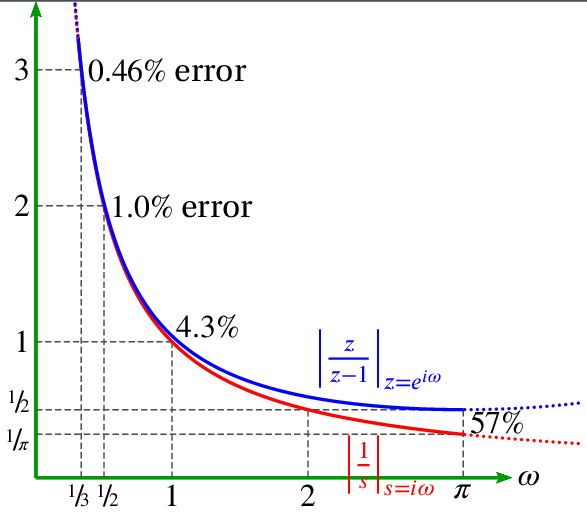
For the DFT, z=eiω. Therefore, the z-transform of y(n)=x(n)-x(n-1) is Y(z) = X(z) – z-1X(z) and:
We can plot the magnitudes of both to compare them:
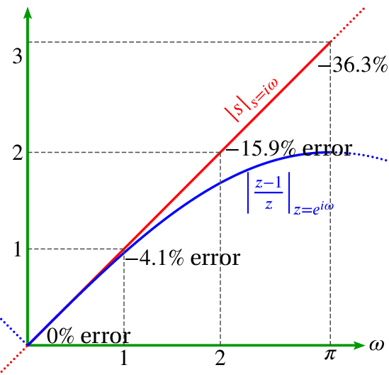
Note that digital differentiation is more accurate at lower frequencies.
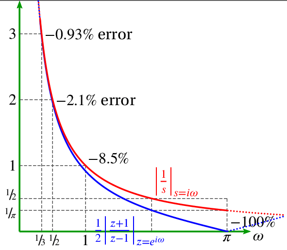
Digital Integration
A similar analysis can be performed for integration. Here, the Fourier transform is -i/iω. The two digital methods are integration using summation and integration using the trapezoid rule.
Integration using Summation
Integration using Trapezoid Rule