Test Types: Random
March 29, 2018
Background
Using VibrationVIEW
Laboratory Exercises
Reference
Back to: VibrationVIEW Syllabus
Real-world vibration is not repetitive or predictable. Consider a vehicle on a roadway, a rocket in take-off, or an airplane wing in turbulent airflow. None of these events have a predictable vibration pattern. The goal of random vibration testing is to create a vibration spectrum to simulate real-world vibration in the lab.
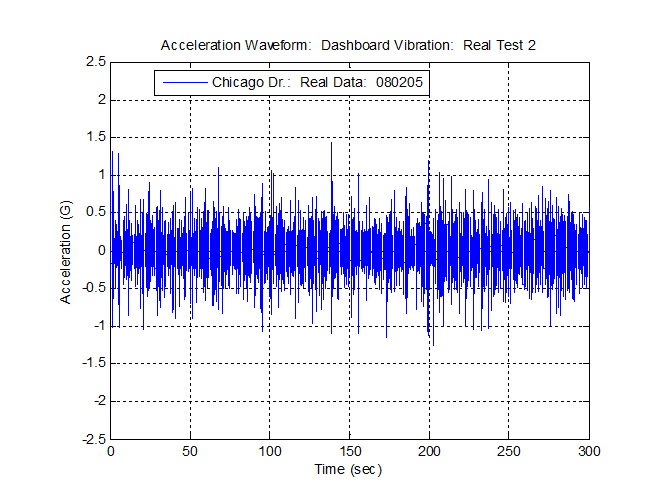
Figure 2.1. Data collected on a vehicle dashboard in Hudsonville, MI.
The acceleration waveform in Figure 2.1 is a recording of the dashboard vibration experienced in a vehicle traveling on Chicago Drive near Hudsonville, MI. The vibration is in no way repetitive.
Random vibration testing is used extensively in the transportation industry. One of the main goals in random testing is to bring the DUT (device under test) to failure.
Random Testing Compared to Sine Testing
How does random testing differ from sine testing? Sinusoidal vibration tests consist of a single frequency at any moment in time. Random vibration consists of all the frequencies in a defined spectrum that the controller sends to the shaker at any given time. Consider Tustin’s description of random vibration:
“I’ve heard people describe a continuous spectrum (random vibration, VRC), say 10-2000 Hz as ‘1990 sine waves 1 Hz apart.’ No. That is close, but not quite correct… Sine Waves have a constant amplitude, cycle after cycle… Suppose that there were 1990 of them (constant amplitude sine waves, VRC). Would the totality be random? No. For the totality to be random, the amplitude of each slice would have to vary randomly, unpredictably… Unpredictable variations are what we mean by Random. Broad-spectrum random vibration contains not sinusoids but rather a continuum of vibration (with differing amplitudes, VRC)” (pg. 234-235).
To accomplish the same degree of testing, multitudes of sine tests would need to be administered, whereas a simple random test would perform it all in one test. Random vibration testing is, therefore, much more efficient and precise.
Random testing is also more realistic than sinusoidal testing. A random spectrum simultaneously includes all the forcing frequencies and “simultaneously excites all our product’s resonances” (Tustin, pg. 224).
During a sinusoidal test, the user may find a resonant frequency for a single part of the DUT first. As the test progresses, another resonant frequency might appear. Exciting resonant frequencies at different times may not cause failure, but failure might occur when all resonant frequencies are excited at the same time. Random testing allows a bandwidth of frequencies to be excited simultaneously, which forces all the resonant frequencies in the band at the same time.
Running a Random Test
The user must develop a random test spectrum to perform random testing. Computer software collects real-time data over a period and then combines the data using a spectrum averaging method. The product is a statistical approximation of the random vibration spectrum.
Traditionally, the new spectrum is then converted into an amplitude probability density graph (PDF) similar to Figure 2.2, assuming most of the data are in the ± 3 sigma range (i.e. Gaussian distribution).
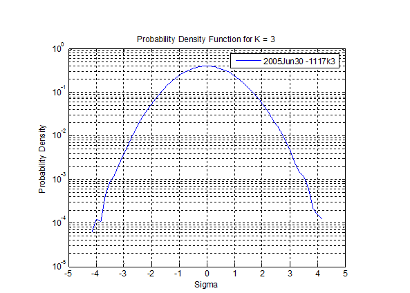
Figure 2.2. The probability density for a light bulb test using Gaussian distribution.
By assuming that the amplitude probability density falls within the ±3 sigma range, much of the real-time data is removed. The acceleration values of extreme magnitude are omitted from the probability density when the traditional Gaussian distribution method is used.
Consequently, present-day random testing methods can be unrealistic because they fail to take the high-level accelerations into account. Furthermore, random testing with Gaussian distribution will take longer to test the product to failure because the high-level accelerations have been omitted.
Random Vibration and the Power Spectral Density
One of the more complex aspects of random vibration is the way the vibration is traditionally displayed. Logically, vibration is displayed in the time domain because vibration occurs over time. However, random vibration is generally displayed in the frequency domain.
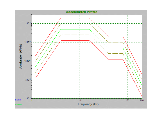
Figure 2.3. Amount of power per unit of frequency as a function of the frequency.
Converting time domain data to frequency domain data is performed using the fast Fourier transform (FFT). For more details on this process, see Kipp, Bill. “PSD and SRS in Simple Terms,” ISTA Conference, Orlando, FL, 1998. Consequently, the random vibration spectrum is displayed as a power spectrum: a plot of acceleration spectral density (typically G2/Hz) versus frequency (Figure 2.3). A power spectrum displays which frequencies contain the power.
According to the ESH Working Group on Blood Pressure and Heart Rate Variability, “The power spectral density, PSD, describes how the power (or variance) of a time series is distributed with frequency. Mathematically, it is defined as the Fourier Transform of the autocorrelation sequence of the time series. An equivalent definition of PSD is the squared modulus of the Fourier transform of the time series, scaled by a proper constant term” (source via web.archive.gov).
The PSD is the result of an averaging method used to produce the statistical approximation of the spectrum, so an infinite number of real-time waveforms could have generated the PSD. Thus, at any time during the test, the PSD cannot determine what forces the DUT is experiencing. Test engineers use the PSD to make an appropriate test profile for the shaker that will come close to the real world vibration the DUT will experience.
Figures 2.4 – 2.7 demonstrate the idea that different waveforms will average to make the same PSD profile graph. The figures display data collected at Vibration Research on June 28, 2005, and June 30, 2005. The acceleration waveforms, although very similar, are different. Additionally, the PSD spectrum from each acceleration waveform is the same even though the data are from different waveforms.
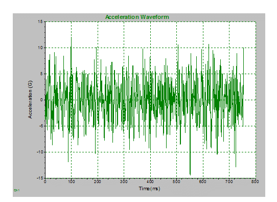 Figure 2.4. The waveform for body and IP profile lightbulb, 2005 Jun 28. |
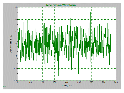 Figure 2.5. The waveform for body and IP profile lightbulb, 2005 Jun 30. |
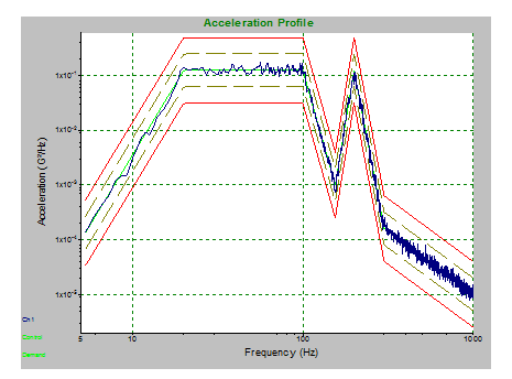 Figure 2.6. PSD spectrum for trial, 2005 Jun 28. |
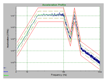 Figure 2.7. PSD spectrum for trial, 2005 Jun 30. |
Random testing is more advantageous than sinusoidal testing but has its disadvantages. Therefore, a more effective method of testing would prove more valuable. To improve upon traditional Gaussian distribution in random testing, Vibration Research has developed a patented technique of kurtosis control called Kurtosion®. With this technique, it is possible to put the peak accelerations that are typically removed back into a vibration test.
Random Vibration and Kurtosis Control
Kurtosis control, or non-Gaussian vibration, is a recent development in vibration testing. Present-day computer software programs collect real-time data over a set period. Then, the data is combined by averaging the spectrum. The product is a statistical approximation of the vibration spectrum.
However, even kurtosis control is not free from limitations. The overall spectrum does not include sporadic vibration events and may discount vibration of potential importance.
Kurtosis control results in a Gaussian distribution of data where the highest peak accelerations are approximately ±3 times the average acceleration. Gaussian distributions omit the highest accelerations and therefore under-test the DUT. The highest accelerations are often the cause of the greatest damage to a tested product.
Gaussian distribution is universally accepted as a legitimate averaging technique. This is, in part, because real-world data is assumed to be Gaussian. However, several studies have shown that real-world data are not Gaussian. (See: Steinwolf, A. “Shaker simulation of random vibration with a high kurtosis value,” Journal of the IEST, May/June 1997; 40,3 and Van Baren, Phil. “The missing knob on your random vibration controller,” Sound and Vibration, October 2005, pg. 10-17.)
Figure 2.8 shows 40 real-world tests in automotive, aeronautical, agricultural, and industrial environments, many of which are non-Gaussian.
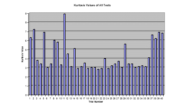
Figure 2.8. Kurtosis values for 40 tests conducted by Vibration Research Corporation. Note the variety of kurtosis values; 23 tests have k>3.3.
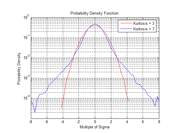
Figure 2.9. A comparison of kurtosis values 3 and 7. The higher kurtosis value includes higher sigma values (higher peak accelerations).
As real-world data is often non-Gaussian, random vibration must be improved so the number of large peak accelerations can be manipulated while the test profile spectrum stays the same. As Bill Kipp said in the 2008 International Transport Packaging Forum™, “Kurtosis control (non-Gaussian vibration) is a means of increasing the amplitudes of the peaks without changing the spectrum shape or the overall average acceleration level” (Kipp, Bill. “New considerations for random vibration testing of packaged products”, 2008 International Transport Packaging Forum™).
Figure 2.9 shows a PDF graph with a typical Gaussian curve in red and a curve with a higher kurtosis containing higher peak acceleration values in blue.
Vibration Research’s Kurtosion
Vibration Research’s patented kurtosis control technique, called Kurtosion, includes the higher peak accelerations and maintains the original test profile and average energies. When changing the kurtosis value, the PSD profile is not affected, but the peak accelerations are significantly higher. Module 2.3 details the differences between Kurtosion and a traditional random test.
Figure 2.10 and Figure 2.11 illustrate how kurtosis control produces a more realistic waveform and PDF than Gaussian distribution. By including the larger peak accelerations in the data, kurtosis control more accurately represents the peak accelerations that occur in the real world. Figure 2.10 displays the PDF of the accelerations of a Cessna’s side window during landing. In Figure 2.11, the acceleration waveforms for an SUV’s dashboard vibration are compared.
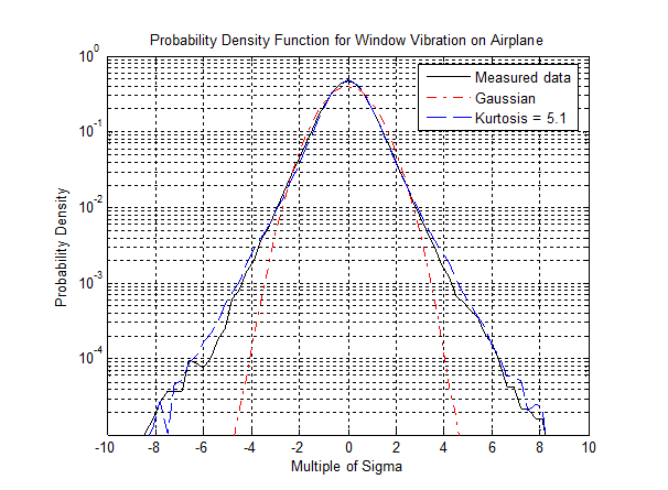
Figure 2.10. Cessna landing in Ludington, MI; side window mounted (16:17. 2005 Aug 5).
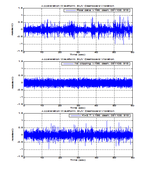
Figure 2.11. Acceleration waveforms for Bravada dashboard vibration on I-196 (9:18, 2005 Aug 5). Measured real-life data, Gaussian (no clipping), and Kurtosis Control (k=5.7) waveforms.
Kurtosis control is a more effective method of conducting random vibration tests because the acceleration waveform more closely replicates real-world vibration. In addition, kurtosis control shortens the time needed to reach failure in the lab environment. This proves beneficial for industries that test products to find points of failure.
Kurtosis Comparison
Vibration Research conducted a simple study to illustrate this point. Seventy-five Watt light bulbs were tested with a slightly modified standard automotive specification. The bulbs were subjected to random vibration until the filaments broke and the bulb burned out. A total of 66 light bulbs were tested, with 22 bulbs at kurtosis levels 3, 5, and 7. The time to failure for each bulb was measured and recorded.
The time to failure for all tests is shown in Figure 2.12 and Figure 2.13. As the kurtosis values increased, the time to failure decreased. The higher kurtosis values include the higher peak accelerations, which are responsible for a more damaging test and shorter testing time. Kurtosis control proves to be a great improvement on traditional random vibration from every perspective.
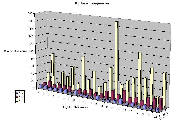
Figure 2.12. Kurtosis comparison of lightbulb failure tests.
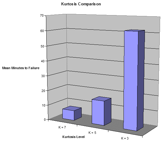
Figure 2.13. Mean minutes of failure versus kurtosis level.
Random Vibration and the Fatigue Damage Spectrum (FDS)
FDS is another new method of random testing. An FDS creates a realistic random vibration test that can be used to inflict a lifetime of damage in a much shorter timeframe. FDS takes a time history file representative of the product’s life. Then, taking multiple levels of acceleration into account, it creates a test.
An example of “levels of acceleration” could be the road surface no which a vehicle travels during its lifetime, such as 80% highway, 10% city streets, and 10% gravel road. Traditional random tests do not differentiate between these levels and either lose the peak accelerations or concentrate on the peaks only. Once an FDS profile has been generated, a time component is applied to scale. For instance, 24 hours of testing could equal 1,000 hours of product life.